The original article was published on May 12, 2025.
Image generation with generative AI models is easy, but I wish creating "good images" was easier too!
Our company has a unique image style which defines bodies and objects while maintaining minimal detail in a specific ratio (reference). Our team embarked on a project to create a text-to-image model that generates images applying this style using only prompts.
This project was initiated to minimize the repetitive image creation work of our in-house designers. Among company design tasks is the work of drawing slightly different images to match situations. We believed that by automating this task, we could create an environment where designers could focus more on creative tasks.
The image below, created following our style, shows the style and level of the final output we desire.
 |  |
As always, making generative AI models consistently create good images wasn't easy. For instance, think of generating an image of a woman holding a "hold the LINE" picket sign, as shown below. An image similar to our style might be generated, but often, non-compliant images would occur too. In fact, the same model was used to generate the two images below, only differing in the hyperparameters set during image generation (we'll explain hyperparameters in more detail later).
| Input | Expectations | Reality |
|---|---|---|
| Draw a woman holding a picket sign! (A woman is holding a picket sign. The sign has the words "hold the LINE" written on it.) | 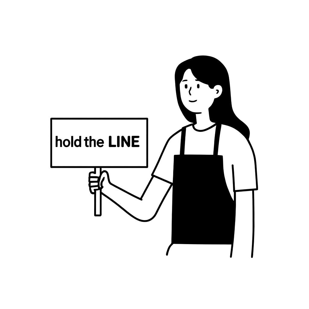 | 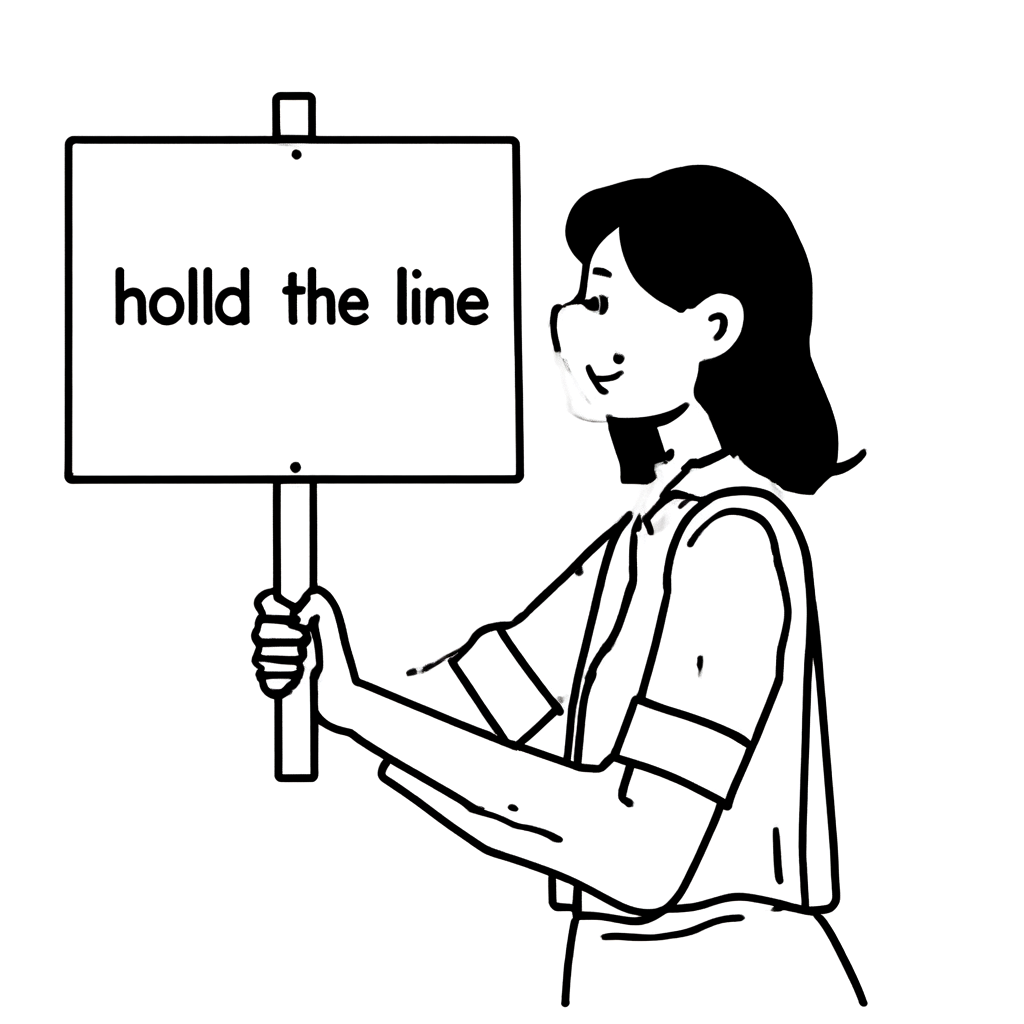 |
Considerations for generating good images
In this post, we'll first explore how to generate images using AI. We will start with the Diffusion model and focus on the Stable Diffusion lineage, introducing several hyperparameters widely used when generating images with the Stable Diffusion model and explaining their features.
To discover how to generate good images, it's typically necessary to generate images multiple times by adjusting a set of hyperparameters. Creating images by varying values within a specific range requires significant effort, so automating this process would be helpful. To automate such tasks, you must first quantify and evaluate what constitutes a "good image". Here, we will introduce some of the image evaluation methods explained earlier (Evaluating AI-generated images (The basics)) and introduce a hyperparameter search method using these techniques. Besides ways to quantify and evaluate images, we will also introduce prompts for hyperparameter evaluation and delve into how they may be used—so stay tuned as we get started.
How AI generates images
Let's briefly look at how generation models generate images, focusing on the Diffusion model and Stable Diffusion model (subsequent explanations are based on the Stable Diffusion model).
Diffusion model
The diffusion model is an approach widely used in image generation, training, and creating images through a diffusion process. The diffusion process systematically removes noise from images to generate high-quality images.
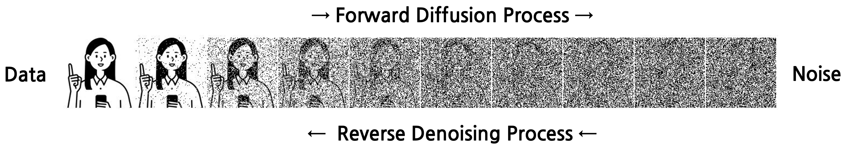
- Forward Diffusion Process: This process involves progressively adding noise to the original image, transforming it into a completely random state. Gaussian noise is added at each stage, using a Markov chain model, with each stage proceeding independently without relying on previous results.
- Reverse Denoising Process: This process involves restoring the original image from the noise-added image. It does so using a trained model to gradually eliminate the noise, recovering a state close to the original image. The model learns the probability distribution of noise removal at each stage, predicting the noise removal stochastically.
Images are created by applying the reverse denoising process to sampled random Gaussian noise.
Stable Diffusion model
Stable Diffusion (SD) is an implementation of the diffusion model. Here's a brief explanation of its features.
Traditional diffusion models apply the diffusion process in the "pixel space", leading to extensive computations when generating large images (for example, 1024x1024 pixels). To address this downside, the SD model applies the diffusion process in the "latent space". While previous diffusion models aimed at reducing noise directly in images, the SD model focuses on reducing noise in the "latent vector" of the image. Latent vectors denote positions in the latent space and may be perceived as embeddings. Generated through encoding by a variational autoencoder (VAE), images decode through the VAE as well.
In text-to-image generation, textual information aids in image generation during the noise removal process via the attention mechanism, while fine-tuning image generation models mainly involves tuning the U-Net, a denoiser.
SDXL and SD3.5 models
In our experiments, we used SDXL (SD-xlarge) and SD3.5 instead of the initial version, SD1. These models, enhanced by increased parameters, are improved versions. (Images attached in this post were mainly generated using SD3.5).
SDXL's structure isn't vastly different from SD, only adding another text encoder (CLIP-G/14), widening its extraction of diverse prompt information compared to the initial SD (SD1).
SD3.5 includes an additional text encoder (T5 XXL) and introduces changes to the denoiser. Learning methods change from a diffusion process to a flow matching method, moving from a diffusion model to a flow model despite its name. The newly adopted denoiser is the multimodal diffusion transformer (MMDiT). As it contains separate modality stacks for text and image and linear layers for each, it increases learnable parameters over U-Net. It doesn't perform calculations separately for self/cross-attention, rather handles attention in a unified block by concatenating each modality.
While diffusion models generate images by learning to add and remove noise, flow models propose that it’s possible to generate images using a simple Gaussian distribution mapped to complex image data distributions. Thus, sampling from a simple Gaussian distribution leads to generating the image data corresponding to it.
When considering how to map a simple Gaussian distribution to actual data, flow matching approaches using a vector field learn transformations within the data space. We'll explain this with the image below.
First, look at the left image (below). Assume a normal distribution (a single peak circular shape) and data distribution (an elongated shape with two peaks) exist arbitrarily in a space. When visualizing the normal distribution on the left transform into the data distribution on the right, imagine moving to the right while gradually extending upwards and downwards. Each space point might undergo change, expressible with a vector field, which flow matching generalizes as learning the vector field.
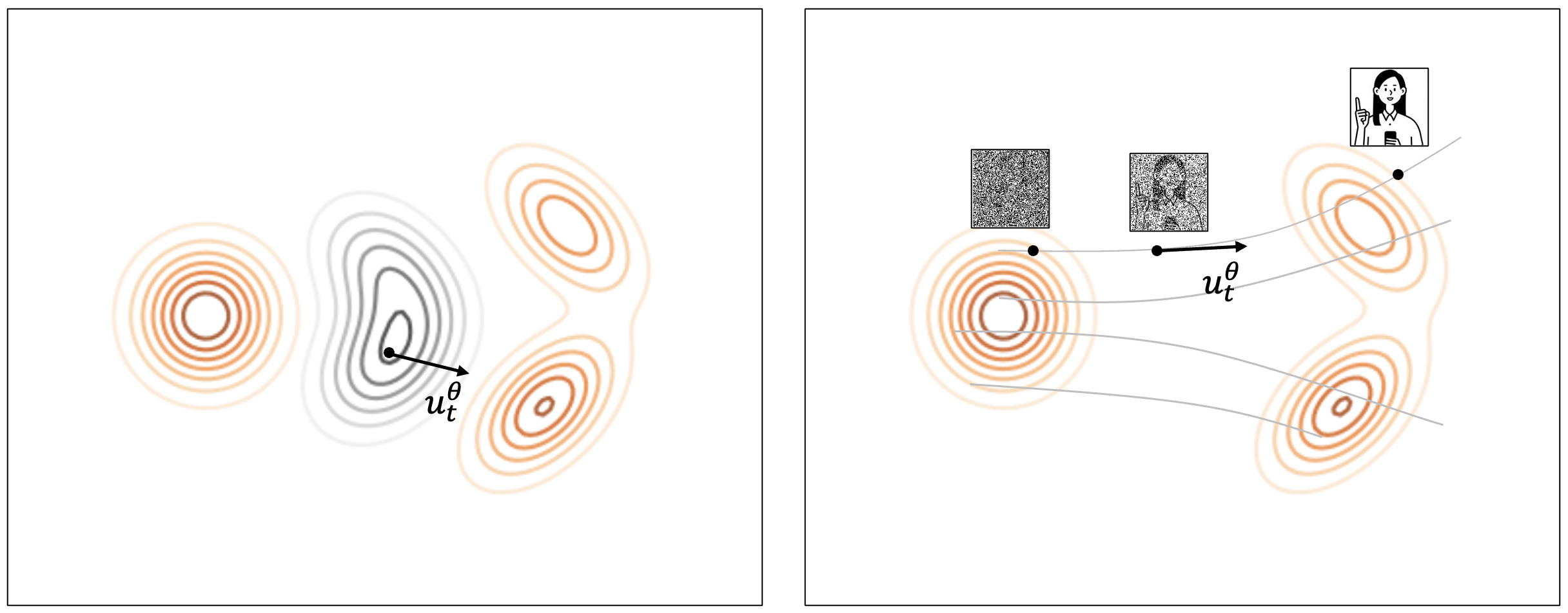
Next, look at the right side image above. In contrast to the diffusion process where it's about reducing noise from random distributions, this involves gradual movements from a sampled random noise to a data point on the right. Therefore, image creation in flow matching entails repeatedly moving a determined distance from a sampled random noise, where direction and distance, called the velocity (), are derived from differentiating the vector field. Thus, flow matching models are deterministic due to providing the same result for the same inputs.
Hyperparameters controllable during image generation and their roles
Let’s introduce the types of hyperparameters used in our experiments and their roles.
Seed, random noise, latent vector
Image generation models receive random noise as input, acting as the starting point in image creation. The seed is an integer value that generates this random noise. With the same seed, the same random noise is consistently generated. Earlier, when discussing Stable Diffusion, the concept was introduced that noise reduction occurs from the latent vector or position in latent space rather than images themselves. Further consideration reveals this includes random noise too, which exists as latent vectors within latent space.
In summary, a seed decides the initial input value for the model, and random noise is its starting input. The distinction lies between the seed being an integer and random noise being a latent vector, but generally, both infer "initial value" depending on context, often used interchangeably. Here, concepts are deliberately separated for use in "searching for a good starting point".
Prompt
Prompts allow adding additional information to image generation models beyond noise. These text inputs are incorporated as text-to-image generation models. During learning, text captions alongside image data offer models contextual insight, refining understanding through “what kind of image adheres to what caption” processing.
While useful for tailored results reflecting user intent, prompts don’t completely control image composition or color, however.
Classifier-free guidance
Classifier-free guidance (CFG) allows controlling the extent to which generated images reflect prompt information. In the noise removal process, both prompt-conditioned and unconditioned/no negative prompt-based noise predictions are utilized. CFG adjusts how much the difference between the two predictions influences the outcome.
Defined as a hyperparameter, a higher value strengthens the prompt-conditioned noise usage, resulting in images more reflective of the prompt. If desired objects fail to appear in the image, adjusting CFG to a higher value enables stronger influence.
Reward guidance
Reward guidance (RG) provides a method similar to CFG to control how much of the prompt’s information reflects in an image. It uses the disparity between the original model’s and a newly fine-tuned model's expressiveness, relying solely on prompt-conditioned noise information. A hyperparameter determines how much this disparity affects the outcome. A higher RG value emphasizes fine-tuned model noise usage, yielding images more inline with trained model aesthetics and styles.
Skip-layer guidance
Used in the SD3 lineage, skip-layer guidance (SLG) utilizes prompt-conditioned noise predictions by comparing total block predictions to those excluding certain blocks in noise removal models (SD3's MMDiT). Within related communities, SLG is reported to mitigate anatomical inaccuracies such as overly many fingers or twisted joints.
Low-rank adaptation scale
Low-rank adaptation (LoRA) is a method for finely tuning large models with fewer parameters. The LoRA scale defines how much influence the learned LoRA parameters exert in denoiser operations. It determines how much fine-tuned information is applied, impacting each denoiser operation, making it interdependent with methods above.
Numerous other hyperparameters relate to image generation, but we focused solely on those mentioned here in our experiments. For SLG, owing to challenges finding an optimal hyperparameter in initial experiments for our fine-tuned model, it was fixed to 0 in subsequent tests. Only remaining three hyperparameters (CFG, RG, LoRA scale) were tested.
This brings us to an important point: manually generating each image through grid search for hyperparameters is an arduous task with constraints in both time and resources, necessitating more efficient methods.
Finding a good starting point
During project progression, we discovered research papers proposing a framework enhancing image quality through seed mining using null prompts (for example: 1, 2, 3, 4). These studies inspired ideas on finding good starting points.
The main idea behind seed mining is to "organize the unique information inherent to each seed, using it to employ optimal seeds during image generation." Empty prompts—strings with zero-length—extract a seed's unique information. Seed mining entails generating images without text conditions to extract features via embeddings or captioning, preparing a candidate list of good seeds. Among these, from earlier explanation, those pondering how integer seeds can yield information may find understanding through the latent vector noise seeded from these integers.
Lacking time to apply mining steps comprehensively, we borrowed only the idea of "judging good seeds". Furthermore, assumptions were made that a good seed would contain all information from prompt text.
Much research advances judgment methods of good seeds (for example: 1, 2, 3). These address subject neglect and subject mixing issues inherent to SD, where prompts might not reflect in images or descriptions of components mix across depicted objects.
The sample image below illustrates subject mixing via the SDXL prompt "a cat and a rabbit". Although seemingly adequate, deeper scrutiny reveals issues; the cat possesses rabbit-like ears, and the rabbit has a cat-like face.
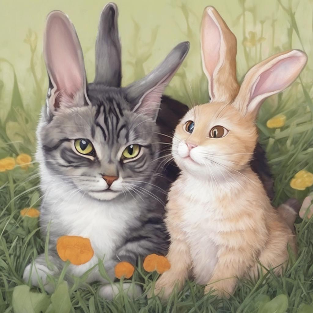
Issues like these arise if the latent vector lacks or erroneously places prompt-related information, addressed by researchers through loss definitions based on utilizing attention maps between latent vectors and text embeddings, proposing vector updates minimizing this loss.
As SD3.5 users restricted by hardware limitations, direct vector updates were challenging, leading us to prioritize loss measurements for seed suitability determination.
The images below vary only by seed change while fixing prompts and hyperparameters. Losses measured within constant prompts and arbitrary seeds within the SD3.5 and a model fine-tuned with our style. Loss values, marked to the fourth decimal, denote exceeding 0.0393 for results achieving the third lowest value: 0.0393.
| Seed | 0 | 42 | 3143890026 |
|---|---|---|---|
| Loss | Greater than 0.0393 | Greater than 0.0393 | 0.0380 |
| Image | 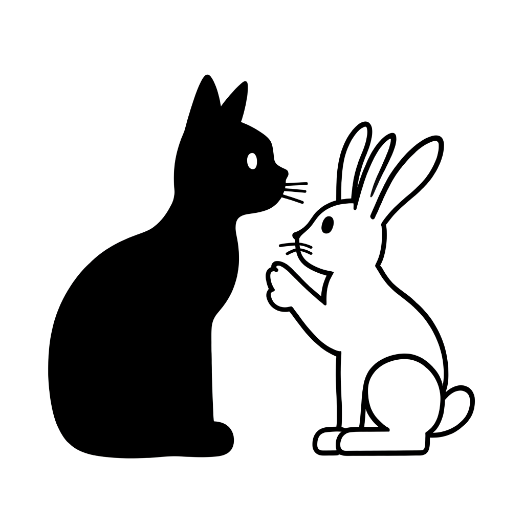 | 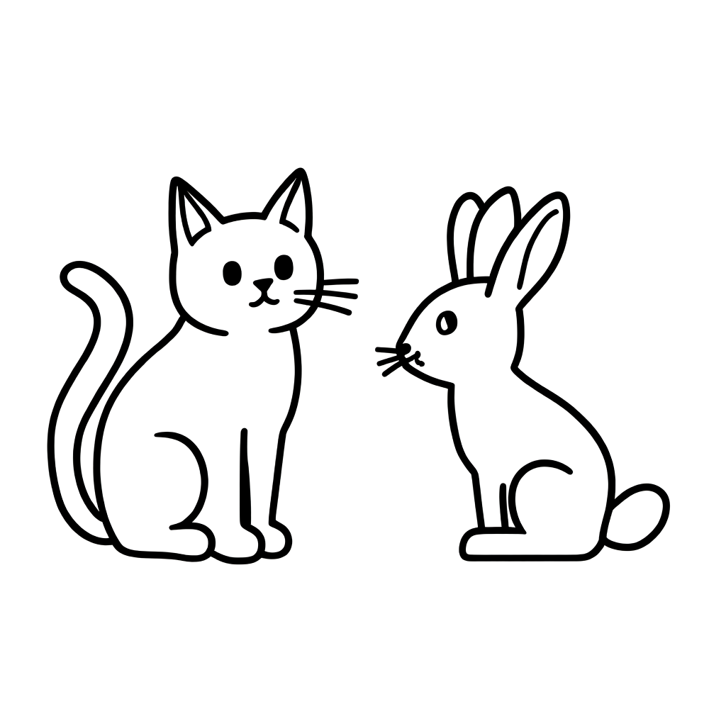 | 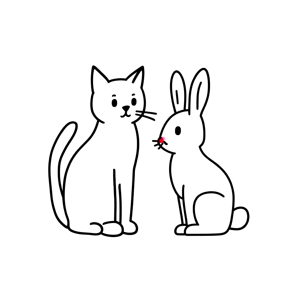 |
| Seed | 2571218620 | 200427519 | 893102645 |
|---|---|---|---|
| Loss | 0.0380 | 0.0383 | 0.0393 |
| Image | 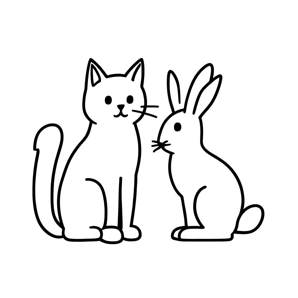 | 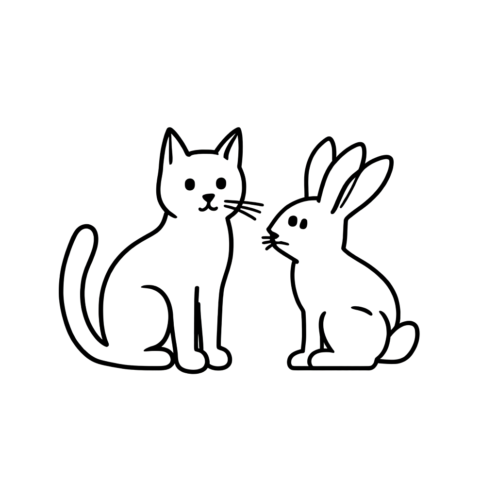 | 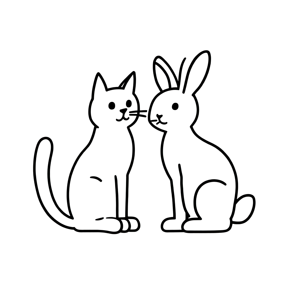 |
From the tables, lower losses generally lead to better image quality, yet this is not a universal rule. As an initial random noise determining value, seed-based loss measurement with prompts doesn’t guarantee enhanced final image quality. We decided to use "3143890026" as a seed for the "a cat and a rabbit" prompt in further tests after this process.
Assessing how good generated images are
While finding a "good starting point", we evaluated generated images manually. Automated processes for mass images necessitated quantifying image quality. In our project, among various indicators explained previously (Evaluating AI-generated images (The basics)), four were used: CLIP score, VQA score, HPS-V2, and Pick score.
Summarized, good images meet the following two requirements:
- The image adequately conveys the prompt's information.
- No strange elements exist, and the image maintains consistency when viewed based on the prompt.
The first condition necessitates measuring the relationship between image and prompt using CLIP score and VQA score, which reflect prompt content inclusion in images.
The second condition assesses image qualitatively using HPS-V2 and Pick score, leveraging learned human preference data from auto-generated image sets over prompts to determine good image quality.
Normalizing indicators with differing scales
Upon deciding these four indicators, an issue arose: differing scales among chosen indicators. All scale definitions lay between 0 and 1, yet raw data measurement varied per indicator. Without normalizing these before calculating averages, tendency bias toward specific indicators could inevitably skew evaluations.
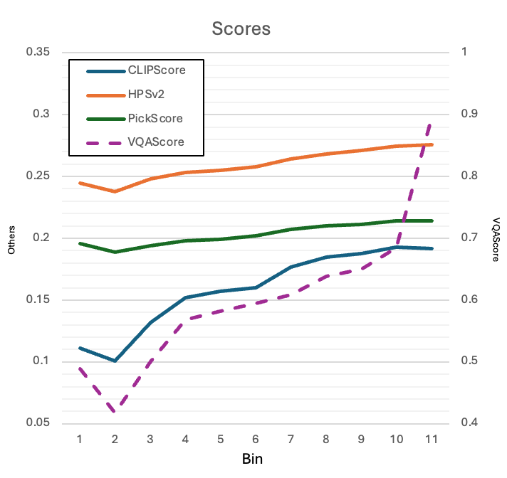
For mitigation, HPS-V2 dataset was used for indicator normalization, incorporating a benchmark evaluating image-prompt pairs human-rated 1-10, experiencing different distributions through stratified sampling for normalizing score value measurements. We set our internal style-followed dataset scores to the highest 11, sorting data into 11 bins accordingly.
Specifically, mean integration occurred through strata evaluations merging each indicator average per rating class. Calculations further incorporated data averaging 1 or 2 ratings, paving the way for standardizing mean and deviation over 11 measured values.
The graph below exhibits ratings associated with generally increasing indicator scores, note that VQA (purple dotted line) versus left standard scaling indices isn’t given precedence. Although evaluators showcased a tendency for lowest scores toward secondary tiers, since prioritizing high scores occurs, we dismissed lower scoring anomalies.
The final calculated indicator averages and standard deviations are as follows:
| CLIP score | HPS-V2 | Pick score | VQA score | |
|---|---|---|---|---|
| Mean | 0.1587 | 0.2591 | 0.2031 | 0.6029 |
| Standard deviation | 0.0323 | 0.0127 | 0.0086 | 0.1248 |
Image scoring averages, post-standardization, reflected this mean value over four evaluators. This normalizing approach continues bearing limitations, as appraising adherence to our style (~10 vs. 11 bin variations) isn't detected thoroughly. With some scores standing apart, assessing style similarity remains complex without extra metrics, addressed momentarily via LoRA scale supplementing.
At default 1, the LoRA scale intricately portrays the learned image traits, retreating to 0 results in no information conveyed. Excessively high values distort image traits, our constraints ensue set parameter adjustments (0.8~1.2), deliberately presupposing precluded models generate images in our style.
Finding optimal values for a function using black box optimization
An automatic image evaluation method is ready. It's time to explore the optimal parameters using the indicators, deploying black box optimization as an alternative method to costly, yet informative grid search. Black box optimization, another name for Bayesian optimization, allows locating function optimum values without knowing the function's internal structure.
Below are examples of black box optimization graphs, illustrating how the black box optimization process unfolds. In the top graph, the red dashed line represents the internal structure-ambiguous black box function graph. The objective is finding the optimum value (maximum here), achievable through functions previously recognized for resembling this unknown function’s shape. Initially, measure the function's value in selected spots(red dots on dashed lines), subsequently approximating it with a characteristic function (the blue solid line). The purple-shaded area displays the predicted confidence interval based upon this function.
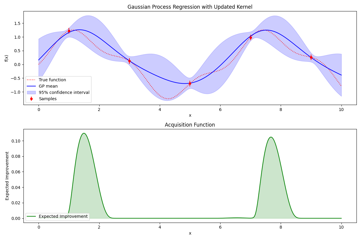
Black box optimization involves minimizing explorations to identify optimal locations. The subsequent challenge is "deciding the next exploration point", aided by the second graph above. The likeliest highest-valued region is a promising candidate. Evaluating unexplored ranges (high uncertainty, expansive light purple spans) may reveal areas harboring satisfactory past outcomes. Expected Improvement (predicted maximum) culminates decisions over the highest likely-value location, facilitating unexplored black box function exploration toward optimal maximum detection.
Defining a function inputting prompt and hyperparameter-generated image scores returns values as a black box function, extending search space through the configurations CFG, RG (1.0~10.0), and LoRA (0.8 ~ 1.2). Bayesian optimization remains an active research field, adopting the library’s default exploratory methods offered per case fundamental. Followed by 3 exploratory searches, and continued 10 further exhaustive probes.
Black box optimization performed with "a cat and a rabbit" prompt
We ran black box optimization with the prompt "a cat and a rabbit", employing the previously explored seed (3143890026). A total of 13 images resulted, with a selected subset arranged in descending score order below. The highest scored image, No. 1, appears of the greatest completion, paralleling eventual image features such as non-compliance or style deviations being probable.
| Number | 1 | 2 | 3 | 4 | 5 |
|---|---|---|---|---|---|
| Image | 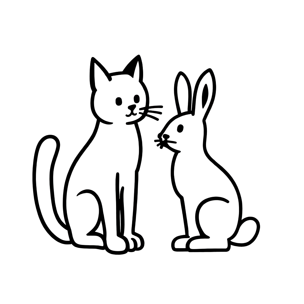 | 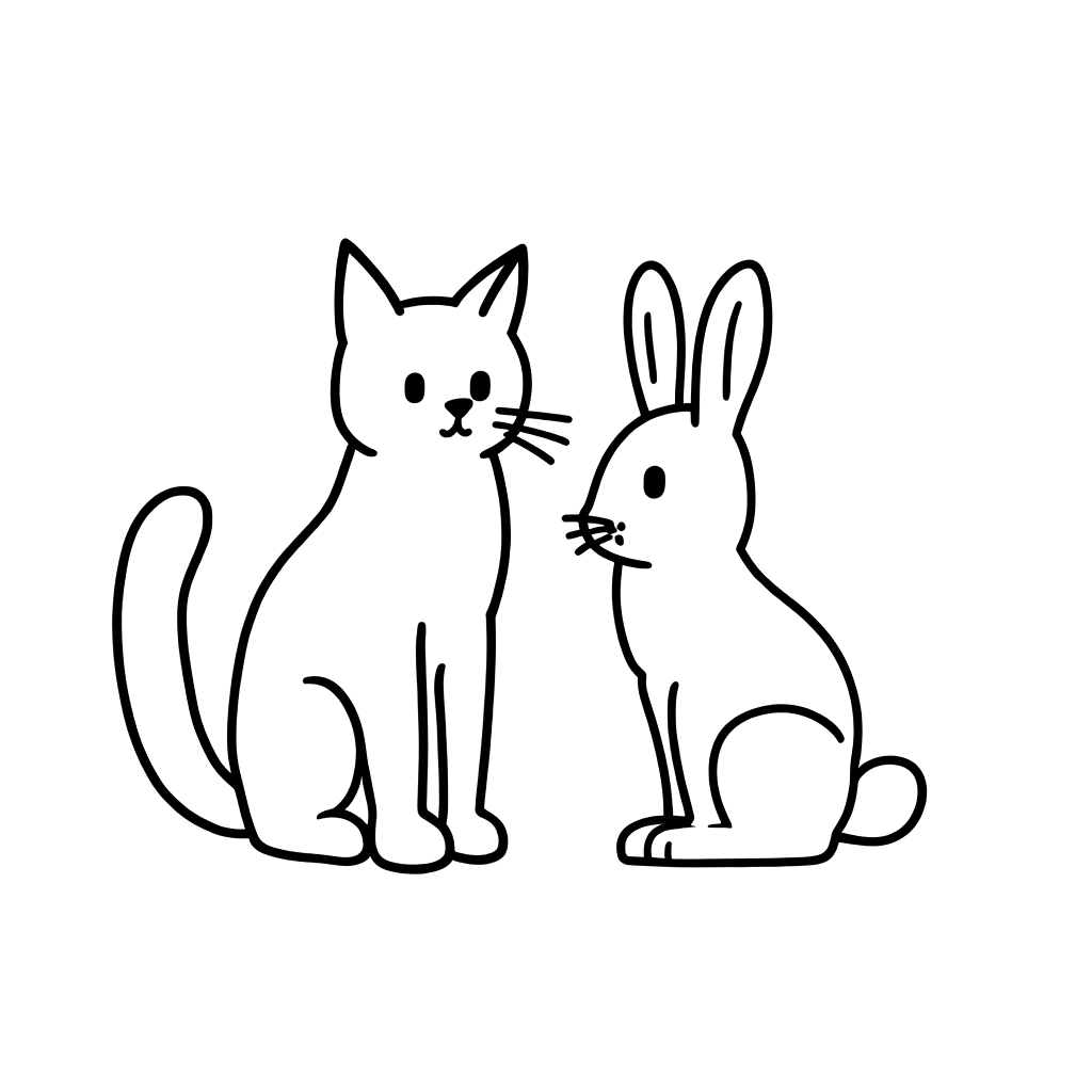 | 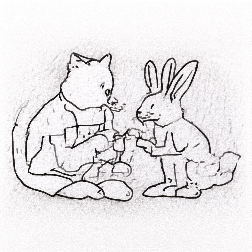 | 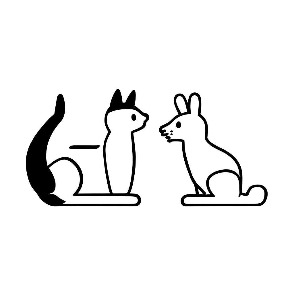 | 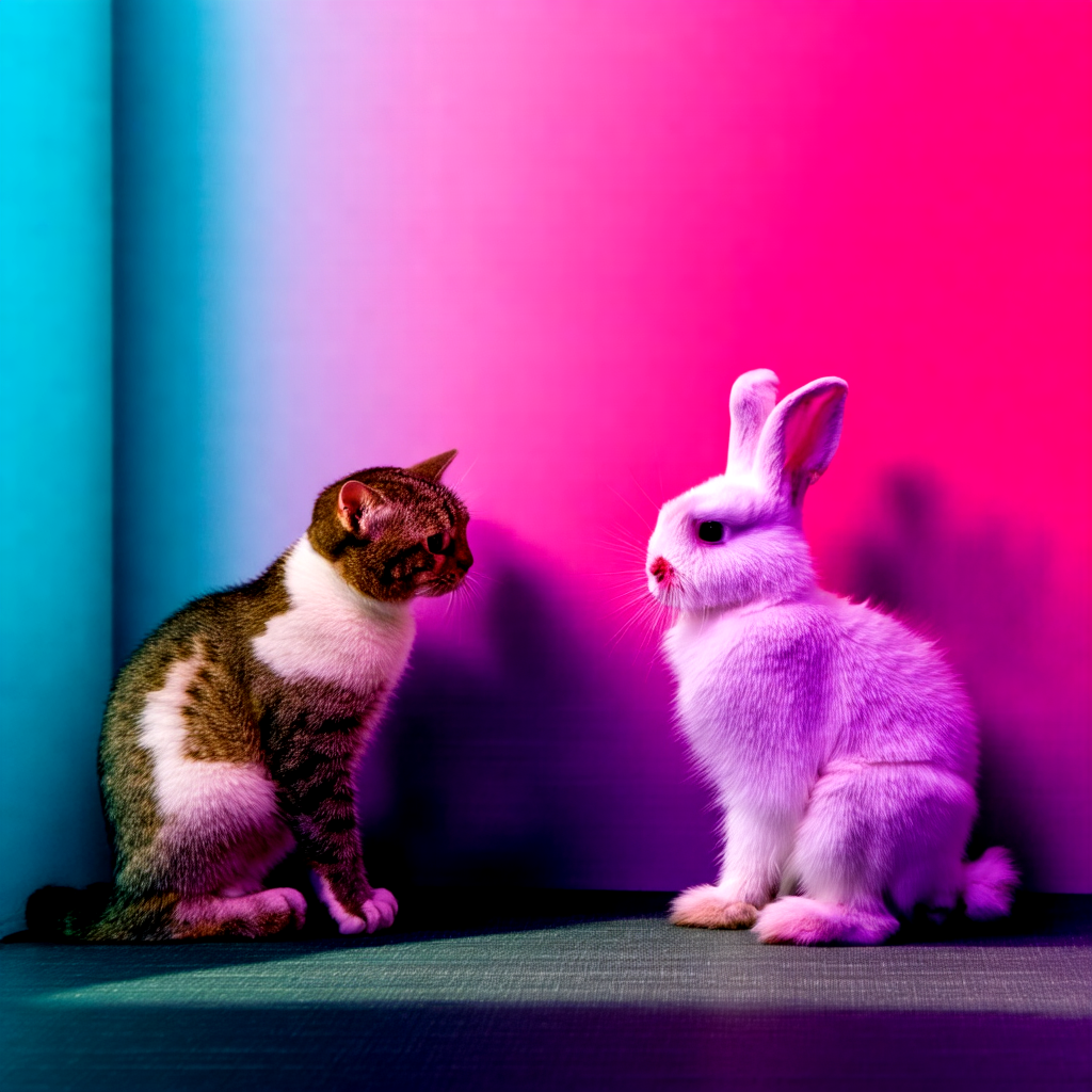 |
| Score | 0.2395 | 0.2386 | 0.2243 | 0.2227 | 0.2088 |
| CFG | 9.1839 | 4.7532 | 1.0383 | 9.9996 | 1.0652 |
| RG | 1.0142 | 1.0010 | 1.0328 | 9.8277 | 9.9207 |
| LoRA | 1.0235 | 1.0881 | 1.0931 | 1.1984 | 0.8468 |
Black box optimization with "A woman is holding a picket sign. The sign has the words 'hold the LINE' written on it." prompt
The same seed exploration method identified seed (2581769315) for this prompt. Utilizing it, 13 images were generated, some ordered below based on descending scores.
| Number | 1 | 2 | 3 | 4 | 5 |
|---|---|---|---|---|---|
| Image | 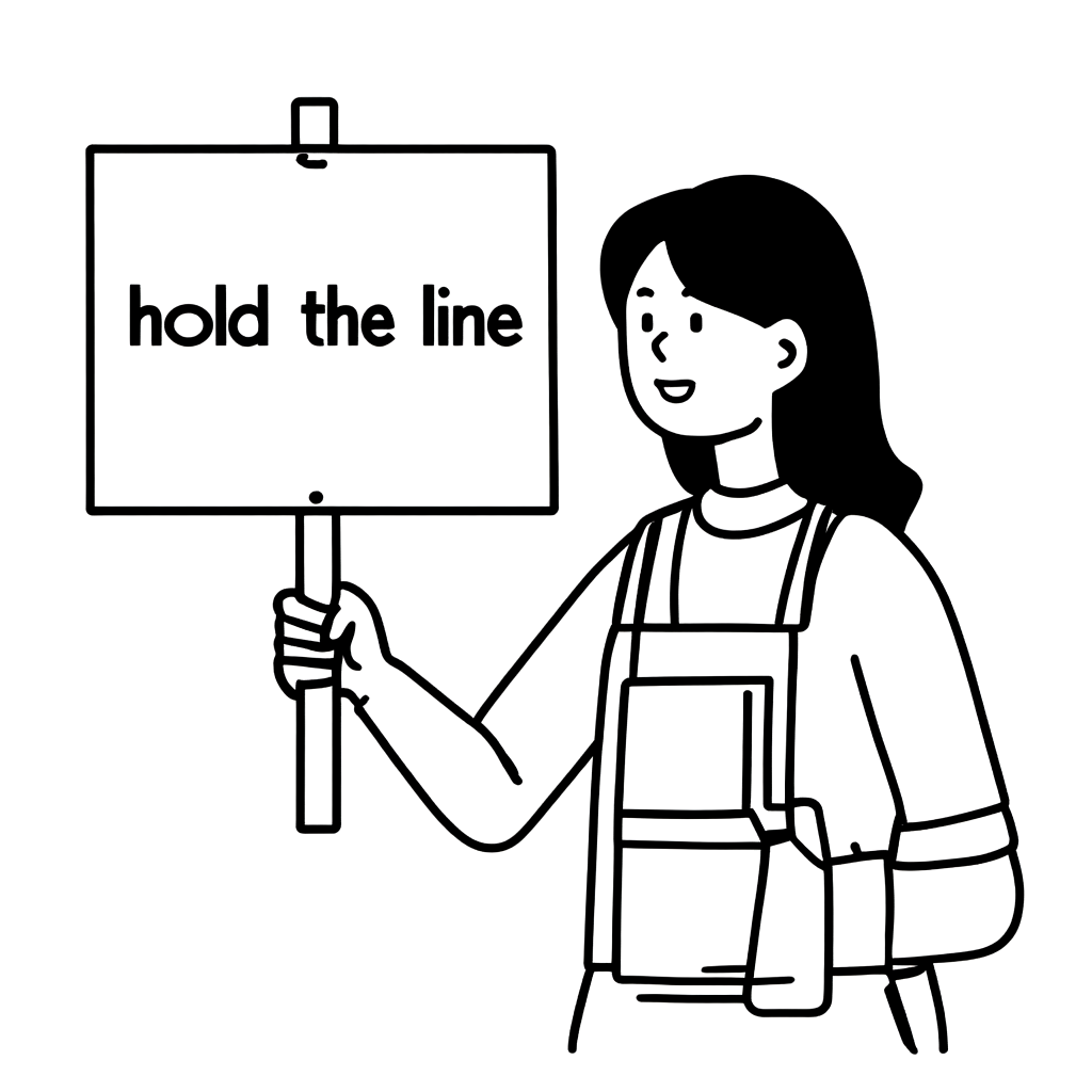 | | |  | 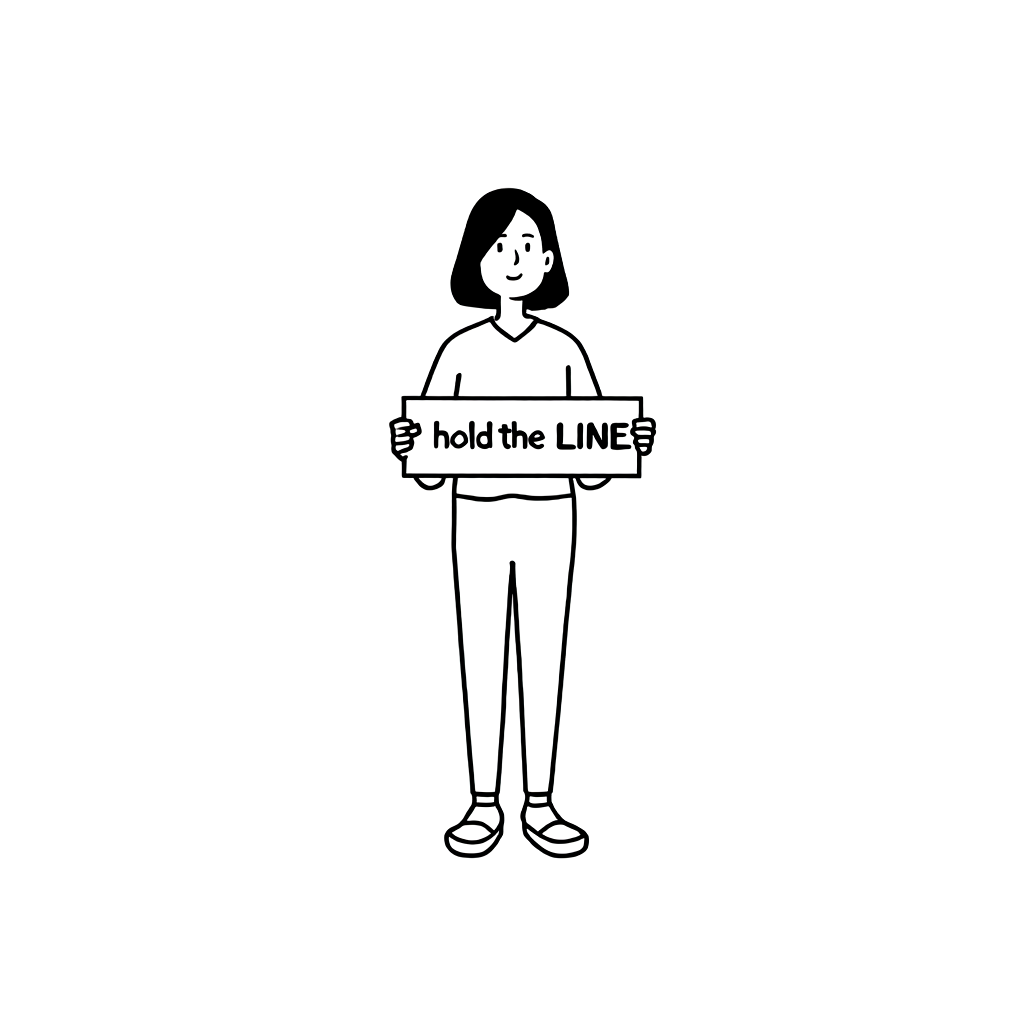 |
| Score | 0.2734 | 0.2681 | 0.2639 | 0.2524 | 0.2497 |
| CFG | 2.7732 | 2.3208 | 3.0985 | 9.9996 | 9.9936 |
| RG | 3.4702 | 2.6763 | 4.335 | 9.8277 | 4.3512 |
| LoRA | 0.8212 | 0.8369 | 0.9913 | 1.1984 | 1.1492 |
The top-scoring image No. 1 appears decent at a glance but can’t be deemed excellent due to the ambiguity around hand and apron expressions. We preferred image No. 3 due to its minimal clothing details and favorable text output.
Expanding further, the higher-score-ranked image No. 2, deemed less normal, indicates image No. 3’s quality exceeds its evaluation. Similarly, ranked fifth image No. 5 outpaces fourth, better representing the face shapes seen in our style. The contrasts underscore needing additional metrics when evaluating adherence to specific styles.
Conclusion: So, was it effective?
Yes, implementing automated image evaluation and hyperparameter search was effective. Specifically, automation reduced manual burdens significantly throughout image acquisition processes, notably improving reliability by statistically based exploration beyond random searches. The resource-saving occurred by lessening the need for deliberation over hyperparameter or optimal seed decisions, directing resources toward business-specific deliberation. Establishing methods determining optimal seeds effectively eliminated one decision-making factor.
However, dissatisfaction lay in the varied traits across generated images within black box exploration. Curbing this diversity could constrict search areas, enhancing probabilities of locating better images. Moreover, deploying CFG, RG, and LoRA scale as black box function inputs in our scenario likely increased exploration difficulty, judging them interdependent rather than independent parameters.
The way forward
Possible future projects could be categorized into the following three:
- Exploration into image evaluation indicators aligning with how well they adhere to our style
- Adoption of image-to-image generation strategies refining control over generated images
- Restraining model-generated image degrees of freedom reducing overall generation space
The latter two topics emerged from ongoing exploration, currently used indices were confirmed short-lined by experiments for style consistency evaluation. Metaphorically heralded text-image generation allows high degrees of freedom regarding image composition and object depiction, thus supplementing image data, aiding controlled outcomes.
The final topic "minimizing generated image freedom scope" reflects differing relevance to the former subjects. Originating from project processes, while aiming at reducing designecting repetitive tasks for predefined images, it's more about in-project reinforcement with finite less freedomed image generation intervention amidst engaging pre-existing repeat-designer-embellishments of objects updated/changed. Beyondmaintaining models yielding less divergent dimension expansions, equipoise could aid improved facility for further modeling refining efforts.
Our continuous development aims endeavoring adaptable AI/ML models bear continued LY employee assistance relevance. Encountering further intriguing themes, we pledge to reconnect. Thank you for engaging with our lengthy exposition.