In this article, we'll share the experience of rebuilding an AI feature store using MongoDB and Spring Cloud Stream. In short, we'll discuss transitioning from a legacy AI feature store system to a new system using MongoDB and Spring Cloud Stream to resolve various issues.
At times, we build systems from scratch for new purposes or inherit existing systems to improve them, or sometimes create entirely new systems that carry on the objectives of existing systems. This often involves dealing with complex and incomplete legacy systems that need improvement and replacement. Development journeys aren't always glamorous like the impressive projects shared on social media. This article aims to share such an experience of building a new system to replace a legacy system, hoping it helps developers facing similar challenges.
This article was co-authored with Saewoong Lee, a DBA from MongoDB, because a key task of the project involved building an unprecedentedly large MongoDB sharded cluster. I hope this will help those interested in MongoDB, especially those looking for real-world experiences related to large-scale MongoDB operations and deployment.
Project introduction
The project aimed to develop a brand-new feature store that could replace the legacy feature store system. A feature store is a system for storing and processing real-time and batch data for AI, ensuring that features can be reused and consistency is maintained. It offers functions such as feature transformation, serving, and storage for AI model development and operation. For more details on the role and utility of feature stores, refer to MACHINE LEARNING FEATURE STORES: A COMPREHENSIVE OVERVIEW.
Previously, we shared the process and outcome of building a high-performance, efficient server for providing real-time embedding data for AI in an article titled How to efficiently handle massive AI real-time embedding (in Korean only). This project aims to develop a system that provides even more types of AI data by combining it with the previous project.
The AI data handled by the two projects are different in nature, and therefore, their system compositions are entirely different. So, even if you haven’t read the previous article, you'll have no trouble understanding this one. However, if you read both, you can see how system structures are affected by data characteristics and the reasons for choosing specific databases.
Legacy system analysis
Sometimes, developers are tasked with creating better systems by inheriting existing legacy systems. In such cases, if one isn’t involved in the legacy system's creation, the first step is analyzing the existing system. The accuracy of this analysis significantly impacts subsequent tasks.
When analyzing a legacy system, it's essential to understand its original purpose, relationship with surrounding systems, infrastructure, and so on. If there are any issues with the system, diagnosing the exact cause is necessary to create a new system that fulfills existing roles while solving problems.
The first step in this project was also analyzing the legacy system environment and issues, which are described below.
The original goal of the legacy system
One of the legacy AI feature store system’s primary objectives was to load and manage large Parquet files. Specifically, it involved downloading large Parquet files for AI services daily or at specific intervals, verifying them, and loading them into the DB within a set time frame for AI model training and real-time service utilization.
While it may seem like a simple data pipeline from the surface, it was a demanding task requiring high performance due to reasons like:
- The Parquet files processed periodically by the system ranged from several gigabytes to hundreds of gigabytes each, needing simultaneous or sequential processing of dozens to hundreds of such files.
- The total data processed daily exceeded several terabytes, with tens of terabytes requiring long-term storage.
- The entire process (Parquet file preparation → download → decompression → validation → DB load → status change and TTL expiration data deletion) had to be completed within a set time frame.
- If processing delays occurred, related subsequent tasks and connected systems could face cascading failures, necessitating stable processing.
- Even during new data load tasks, the service had to handle real-time requests without interruption, maintaining response times within a standard level.
In conclusion, the project’s core challenge was designing an architecture that satisfied all three requirements of large data processing, strict time constraints, and real-time response.
Analysis of legacy system issues
While the legacy system operated meeting the goals mentioned earlier, it had some issues, categorized into server and application configuration problems and constraints related to the primary DB, TiDB.
Server and application configuration issues
The first issue with the legacy system was inefficient use of server resources due to server and application configuration. The servers selected during legacy system development were high-cost machines with disproportionately large memory compared to CPU because of the incorrect approach to the Parquet files discussed below, all centrally deployed in a single node pool. Despite using numerous high-spec servers in this way, the application servers weren't fully utilizing their resources. This led to limitations in deploying various types of pods in the Kubernetes environment, with memory being surplus and CPU lacking, creating inefficiency.
To solve this problem, fundamental improvements to the infrastructure structure were needed. It was possible to make partial improvements by returning some equipment, adding new servers, and dividing the node pool, but this was not a fundamental solution and had evident limitations. Ultimately, reverting all expensive hardware and transitioning to smaller VM-based nodes with standard CPU/memory ratios was necessary to significantly reduce infrastructure costs and secure operational flexibility. For uninterrupted service, constructing a new node pool separately and transferring was the practical choice.
TiDB performance limits and application bottleneck
The legacy system used TiDB as the main DB, and inefficient implementations in application code were attempting to bypass or endure TiDB's writing performance and scalability limitations. This increased system complexity and deteriorated the overall project quality.
Handling exceptional situations
The legacy system was vulnerable to failures with large file processing tasks and had difficulty responding to exceptional situations. It repeatedly downloaded, decompressed, validated, and inputted dozens to hundreds of large Parquet files into the DB daily. If an error occurred during file processing, there was no way to track the precise status or automatically retry, requiring manual intervention. This increased operational burden and posed a potential risk to system integrity.
Issues with the used DB (TiDB)
The issues of the legacy system listed below related to TiDB may stem from TiDB’s characteristics and limitations, or they may be due to the configuration method. Therefore, generalizing the problems mentioned here as issues with TiDB overall is inappropriate.
However, our experience could serve as practical reference material for others experiencing similar difficulties in similar environments. Especially if you are considering points during system design or DB selection, I recommend reading through this article.
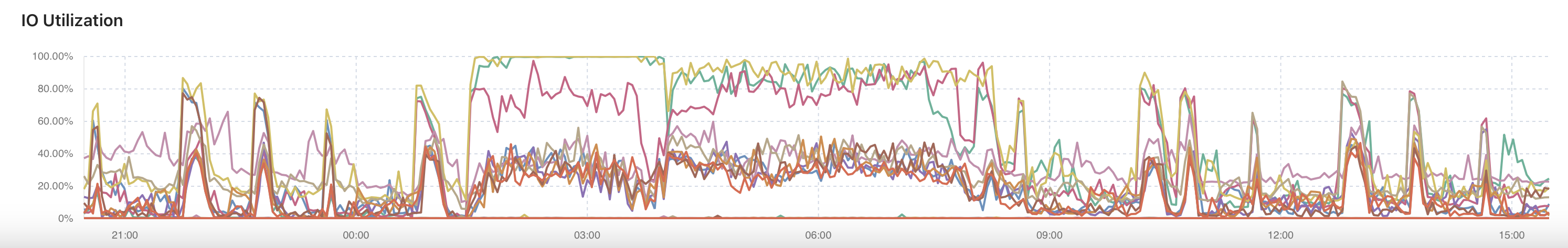
The first problem was the need to distribute the load.
When the legacy system experienced large volumes of new data entered daily and hourly, TiDB’s CPU and I/O usage approached its limits, causing issues in processing service requests. TiDB uses the Raft consensus algorithm, with the leader node handling write requests, then propagating logs to follower nodes to ensure data consistency. Since both read and write requests are handled by the leader node, the load on the leader node rapidly increases during large write operations, potentially significantly decreasing service response speeds, and possibly causing a system crash. If a crash occurs, the leader election process adds extra burden, negatively impacting service stability.
To solve this, read and write operations needed to be separated and handled on different nodes. Generally, in DBs that support replication, write requests are handled by the leader node while read requests are distributed to replica nodes, effectively distributing system load. Starting from the version that supported the follower read function {reference}, TiDB also partially distributes the leader node’s load by processing read requests on follower nodes. However, there seemed to be no consideration of load distribution when the legacy system was originally built, and it wasn’t feasible to take action after inheriting it.
The second issue was that the legacy system’s TiDB couldn’t be considered complete HA (high availability) configuration.
Even with optimal infrastructure environments, various issues such as hardware problems can occur during operations. Thus, HA configurations for infrastructure like DB and servers are essential. Depending on the type of DB, HA configurations automatically process everything from fault detection to its response in an instant, with users barely noticing any fault or briefly encountering disconnected access. However, without HA configuration or if the configuration is incomplete, some aspects of detecting and responding to faults fall to humans, which can be unfavorable in terms of speed and accuracy.
Also, although rare, if problems occur simultaneously with secondary devices even in HA configuration, or if natural disasters damage the equipment, data must be securely backed up, or other recovery means and scenarios must be prepared. Depending on how well-prepared you are for various fault scenarios, recovery time can range from seconds to days, or recovery may completely fail. The legacy system was internally assessed as being far from the perfect point we envisioned, thus becoming a significant reason for deciding to replace it with another DB.
The third issue was the lack of a specialized TiDB team and DBA.
TiDB is relatively less staffed compared to traditional major DBMSs. Thus, it is uncommon for a dedicated TiDB DBA or professional organization to be available. Although the situation during the original legacy system’s development is unknown, the state at the time of inheritance was a substantial burden, contributing to the decision to adopt another DB to replace TiDB.
The legacy system’s issues could be categorized into application and DB parts, and the solutions were also divided into two branches. First, we'll describe how we resolved the application issues, followed by the part where we built and optimized a large-scale MongoDB sharded cluster to solve issues stemming from TiDB.
Resolving legacy system issues 1: Solving server and application problems
Before solving server and application problems, we examined the fundamental reasons for the previously introduced issues. We aimed to understand the core of the problems to derive solutions from this process.
Root cause: Incorrect approach to Parquet files
Large Parquet file data, which can reach hundreds of gigabytes, requires a strategic approach and proper handling, but the legacy system design didn't reflect that. While efficiency is key in processing data, merely assigning high-spec servers to resolve the problem was the fundamental reason. When asked, "Why did you request and assign high-spec servers?" someone familiar with the legacy system history responded, "Since the Parquet files are quite large, it was assumed they'd load in memory for processing. Hence, high-spec servers with large memory were put in place."
To understand why this approach was inappropriate, it's crucial to examine what a "Parquet file" is.
Parquet files are columnar-based formats designed for efficiently storing large data and enabling fast queries. Each column is stored and compressed individually, allowing selective column reads for excellent I/O performance. Moreover, data is stored in row groups, and multiple processes can read data in parallel, with write operations also distributed across multiple files in distributed environments.
As evident from these characteristics, the original design purpose of Parquet is parallel processing optimization. Therefore, it’s designed to allow file splitting into pieces for parallel reading and writing. Unfortunately, the legacy system's approach focused solely on Parquet file size, opting to increase server memory without considering these characteristics. Such an approach was inefficient as it processed large Parquet files by loading them into memory all at once.
An efficient method for processing Parquet files relies not on high-spec servers but on parallel file partitions for reading and writing, maximizing their characteristics.
The key to solving the problem: Exploiting Parquet characteristics with divide & conquer
Divide and conquer is a classical algorithm strategy where a large problem is broken down into small, independent subproblems. Each part is resolved, and results are combined to solve the entire problem. This concept is beneficial in large-scale data processing, and Parquet naturally fits this divide-and-conquer approach. Here’s a breakdown of the process with Parquet:
Divide: Parquet stores data in internally partitioned row groups, allowing physical data separation while logically managing it as a single dataset.
Conquer: Partitioned row groups or files can be processed independently, allowing multiple processors to analyze data in parallel.
Combine: Results from analyses are recombined to form the total output, similar to a divide-and-conquer algorithm’s final stage.
This process resembles the process in divide-and-conquer algorithms, where problems are divided into subproblems, each solved simultaneously, and results are combined to find the solution. Parquet’s characteristics, such as reading-optimized selective column access, columnar storage, and internal partition structure (row group), fit very well with a divide-and-conquer strategy. Such Parquet file exploitation allows naturally “dividing the data, splitting the process, enhancing performance”. In large-scale data situations like this one, reading, writing, and processing performance improvements are maximized.
Kafka as a divide-and-conquer middleware
As explained above, divide and conquer is a strategy to break down large problems into smaller pieces, resolve each of them independently, and combine the results to address the whole issue. Kafka serves as an apt tool to technically implement this strategy.
Kafka’s core concept of topics and partition structures physically divides the data. Partitioning a topic into multiple partitions allows each to handle messages independently and enables parallel consumption. This setup closely resembles a structure where a large data flow is divided into small units to be simultaneously conquered.
Kafka embodies a practical implementation of the divide-and-conquer strategy through features like:
- Retries: Kafka provides a retry mechanism that allows reprocessing of failed messages during consumption. It facilitates easy recovery from failures while preventing widespread system disruption.
- Reprocessing: Kafka stores messages on disk and can be re-read based on offset, enabling retroactive data processing when consumer logic changes or new consumers are introduced.
- Concurrent processing adjustment: By adjusting the number of partitions and altering the number of consumers handling each partition, it's possible to flexibly tweak parallel consumption. More instances can increase processing speed for high-throughput pipelines, while fewer resources can target less intensive ones. However, the number of partitions can't be reduced, and if the partition count is less than the consumer instance number, some consumers may remain idle.
By tapping into these features, Kafka becomes more than just a straightforward message queue, transforming into the practical execution entity of divide-and-conquer, allowing complex systems to be broken down into manageable units for stable processing. Kafka is an ideal middleware for managing large-scale data flows, real-time processing, resilience, and recovery against failures in a decentralized structure.
Kafka-based system design and abstraction level considerations
When configuring applications based on Kafka, we had three primary abstraction level choices:
The first was Spring Kafka, which involves coding Kafka's producers and consumers directly. With precise control over message processing scenarios, this approach allows detailed configuration of internal mechanisms, making it suitable for high-performance or HA situations. However, having developers handle more aspects of coding and configuration increases development and operational effort.
The second option was Spring Cloud Stream. This is a Spring-based messaging abstraction framework that simplifies application logic composition on message systems like Kafka or RabbitMQ. It facilitates easy implementation of stream processing using annotations without complex binding configurations and allows for state storage, retry, and window processing integration with Kafka Streams. However, controlling internal operations completely is challenging.
The third option was Spring Cloud Data Flow (SCDF). It’s a stream orchestration platform based on Spring Cloud Stream that allows visual pipeline construction and easy management using operational tools.
In the development's initial stage, SCDF was chosen because its visual pipeline configuration and operating convenience stood out, allowing quick startup. However, repeated tests of hypothetical failure scenarios revealed an intermittent issue where processes froze and UI stopped recovering correctly upon failure in processing stages, remaining suspended. Such frozen states required manual confirmations and resolutions, highlighting clear limits in reprocessing logic and state recovery during failures. Fortunately, we identified this issue early through pilot tests at the adoption stage, reaffirming the importance of selecting appropriate tools during system design, considering not just specifications or features but also fault response and operating environments.
Ultimately, to enhance the system’s stability and reliability, we transitioned to directly configuring streams with Spring Cloud Stream. Although this approach was initially more complex than SCDF, it allowed precise handling of fault response logic, deemed more effective for securing system stability and reliability. While I could have opted for Spring Kafka, which I have the most personal experience with, we aimed to achieve both rapid development and stability assurance by taking an abstraction layer higher using Spring Cloud Stream.
Composing a Parquet file loading stream pipeline
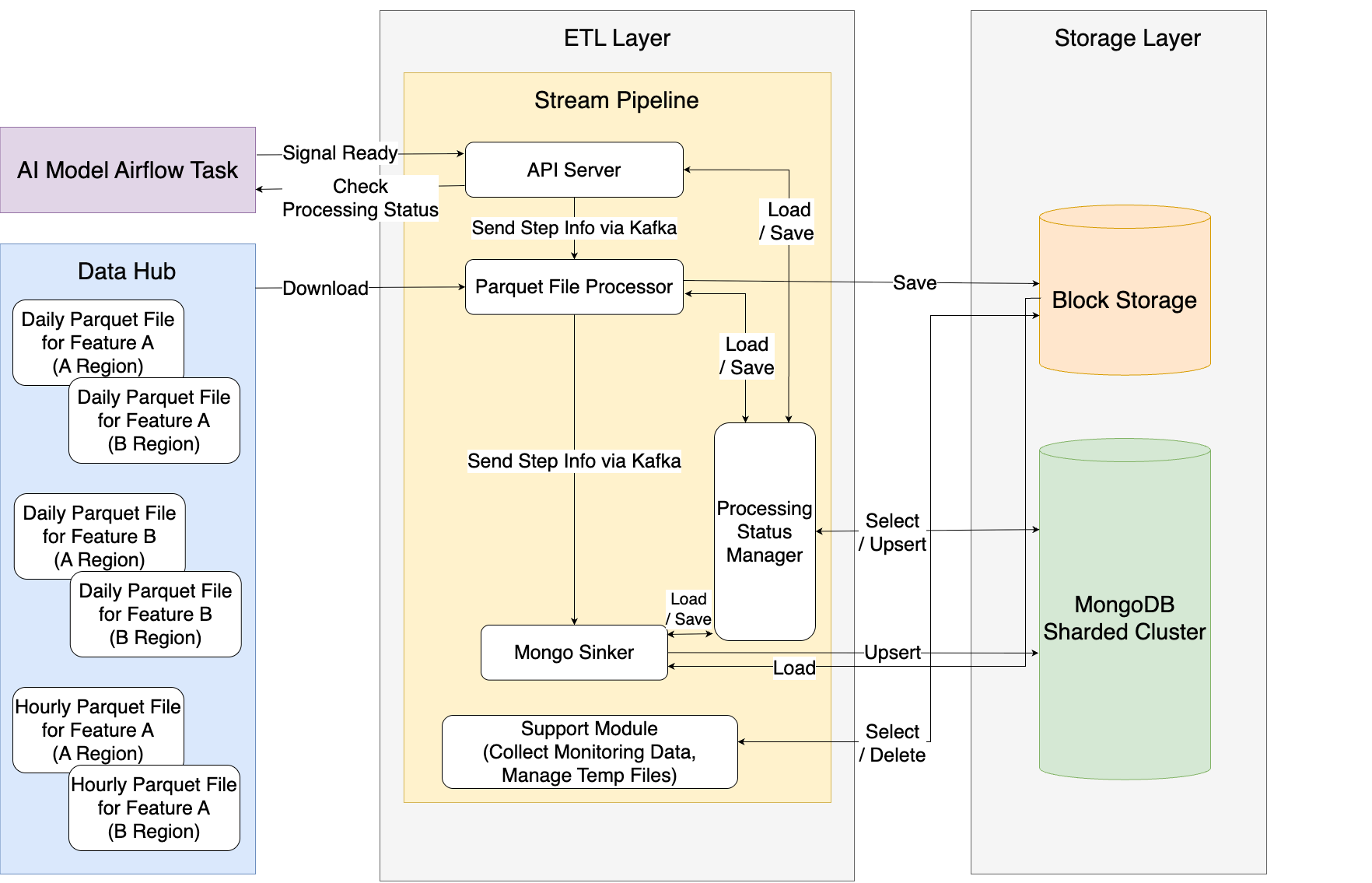
The pipeline was composed of the following modules:
| Module name | Role | Description |
|---|---|---|
| API |
| The process begins after verifying conditions upon receiving a start signal and provides processing status externally. |
| ParquetFileProcessor |
| Parquet files are distributed for parallel downloads, detecting anomalies. After download and verification, processed files are saved in separate block storage, not in the node's storage. It is also the starting point for partitioning and adds information needed for subsequent tracking. |
| MongoSinker |
| It reads Parquet files in parallel from block storage, parses them, and stores them in MongoDB. |
| ProcessingStatusManager |
| It collects the progress status of the entire pipeline and checks for anomalies and consistency. |
| Support |
| Manages files temporarily stored in block storage and provides various metrics. |
From the viewpoint of Spring Cloud Stream, the advantages of this configuration are as follows:
- Loosely coupled modules
- Because each module sends and receives messages via Kafka in a loosely coupled form, each can be developed, deployed, and expanded independently.
- Easy and fast scaling out
- Each module can be executed in parallel as a separate instance.
- It is possible to start scaling individual modules based on their current state, reducing the burden even in situations where uninterrupted service is a premise.
- Infrastructure cost reduction effect
- Some modules consume more CPU, while others consume more memory. Using the Kubernetes environment, we can mix and place applications divided by function based on performance requirements to improve overall node efficiency.
- During scaling or reduction, resources can be allocated based on each module's performance consideration, ensuring no waste.
- Fault isolation and resilience
- Tuning the commit timing allows retries without data loss, even in fault occurrence.
- Processing partition-based isolated data step by step prevents the propagation of partial faults, and in the worst-case, situations where the entire dataset becomes unusable do not arise.
- Easy monitoring and traceability
- Each stream point can be easily monitored, and logs can be traced for quick problem identification.
The following image graphically represents the Parquet file loading stream pipeline's module configuration.
Efficiently placing pods on smaller conventional VM
Initially, we configured all VMs with low specifications with normal CPU and memory ratios, then efficiently mixed and placed various function-specific pods on each VM.
The resource settings for ParquetFileProcessor are as follows:
resources:
  limits:
    cpu: 3500m
    memory: 7400Mi
  requests:
    cpu: 3500m
    memory: 7400Mi
The resource settings for MongoSinker are:
resources:
  limits:
    cpu: 1650m
    memory: 3600Mi
  requests:
    cpu: 1650m
    memory: 3600Mi
The strategy where requests and limits are the same, as shown above, is employed when I/O and CPU usage are high, such as in Parquet file processing, where predictable performance is needed through stable resource isolation. Parquet file processing heavily focuses on CPU usage during column-based decompression, decoding, filtering, etc., and distributed processing needs a guaranteed level of resources per container for optimal efficiency. Applying this strategy grants guaranteed QoS to the pod in Kubernetes, ensuring stable operation during resource competition situations. It allows the scheduler to allocate resources accurately, maintaining consistent processing without performance degradation or resource throttling during Parquet file processing.
Inserting retry logic in each stage of stream processing
In Spring Cloud Stream, when an exception occurs during message processing, retry attempts can be configured, and if it still fails after retries, it can be directed to a DLQ. Retry configurations include:
maxAttempts: maximum attempt countbackOffInitialInterval: initial retry wait time (ms)backOffMultiplier: multiplier for increasing wait times between retriesbackOffMaxInterval: maximum wait timedefaultRetryable: retry possibility for default exceptions
The below setup configures a maximum of 10 retry attempts upon an error during message processing. The first retry takes place 1.5 seconds later, with each subsequent attempt increasing the wait time by 1.8 times, capped at a maximum increase of 12 seconds to avoid excessive delays effectively.
    stream:
      bindings:
        downloadParquet-in-0:
          consumer:
            max-attempts: 10
            back-off-initial-interval: 1500   # Initial wait time 1.5 seconds
            back-off-multiplier: 1.8          # 1.8x increase
            back-off-max-interval: 12000      # Maximum wait time 12 seconds
Listing the actual retry intervals results in [1.5 seconds, 2.7 seconds, 4.86 seconds, 8.75 seconds, 12 seconds, ... keep at 12 seconds]. This progressive backoff strategy aims to restore messages stably during fault occurrence without imposing undue burden on the system. When designing retry logic, not only must the retries function correctly during exceptions but ensuring no duplicate or corrupted data generation through multiple reprocessing is key. Strict adherence to idempotency is crucial for this assurance.
Resolving legacy system issues 2: Establishing a large MongoDB shard cluster
We previously talked about solving server and application-side problems in the legacy system. Now let's discuss establishing a large-scale MongoDB sharded cluster to replace TiDB, considering various factors while applying it to the application (note this article was written based on MongoDB version 6.0.14).
Selecting a MongoDB architecture
The first consideration when adopting MongoDB is deciding on its architecture. The choices are MongoDB replica set and sharded cluster configurations. Each has different objectives and characteristics, so choosing carefully based on service scale and data processing traits is vital. From the perspective of someone who’s used both configurations, it almost feels like these are two entirely different DBs due to their architectural differences. Let’s look at each briefly.
Firstly, the replica set is MongoDB's basic setup to ensure high availability and data integrity. It consists of one primary node and two or more secondary nodes, promoting a secondary node to primary if the current primary fails. Because the same data is replicated across nodes, data consistency is guaranteed. It’s relatively simple to operate, but there might be limits in handling large traffic since all write operations focus on the primary node.
A sharded cluster, on the other hand, constructs to store and process large-scale data in a distributed manner, with datasets distributed to multiple shards based on shard keys. Each shard is independently organized into replica sets, dispersing read and write traffic across nodes. This allows horizontal scaling and the efficient handling of massive data. However, the initial shard key design needs careful consideration, and operating complexity is much higher than the replica set, suiting large-scale systems where data expansion is necessary.
The following table compares MongoDB replica sets and sharded clusters.
| Aspect | Replica set | Sharded cluster |
|---|---|---|
| Primary purpose | Data integrity & reliability via replication | Designed for horizontal scaling and large data processing |
| Data storage method | Replicates data across all nodes | Data distributed across shards based on shard keys |
| High availability | Provided (auto-switching on primary failure) | Provided, with shards/config servers independently set up as replica sets |
| Read load distribution | Secondary usable | Multiple shard secondaries usable |
| Write load distribution | Focused on primary node | Shard-based write load distribution possible via shard key |
| Data distribution | None (all data replicated) | Data divided by shard key among shards |
| Scalability | Vertically-focused (scaling up) | Supports horizontal scaling (scaling out) |
| Operational complexity | Low (simple structure) | Relatively high (requires managing complex settings) |
| Fault recovery | Simple and quick | Relatively complex but offers the advantage of localized fault scope |
| Cost | Relatively low | High due to complex architecture and operational burden |
| Suitability cases | Medium to small scale, systems prioritizing stability over read loads | Fitting for large-scale data management, requiring high-speed read/write; in some scales, it’s the sole option |
For the following reasons, a sharded cluster was selected for this project:
- The project’s required data scale and performance levels couldn’t be met with replica sets.
- A professional MongoDB team handled both setup and operation, reducing concern about difficulty and complexity in setup and operation.
- AI data demands frequent expansions. Hence, a sharded cluster was apt for horizontal scaling at relatively lower costs over vertical expansion; there are exact limits. Vertical expansion has clear limits despite investing heavily in CPU and memory.
- Both configurations support HA and fault recovery.
Once MongoDB’s sharded cluster was chosen, factors like shard key selection, initial chunk numbers, large-scale data deletion strategy, load distribution strategies, application client settings, and Oplog file optimization needed reviewing. Let's look into each focus area.
Choosing a shard key
A sharded cluster's performance and stability largely depend on shard key selection. Changing shard keys once set is challenging. Before MongoDB 5.0, online changes were impossible, and even post-5.0, the ReshardCollection command allows online changes, careful design remains crucial.
The key elements to consider when selecting shard keys are presented in the table below.
| Aspect | Description |
|---|---|
| Cardinality | Select a key that distributes data evenly. |
| Immutability | Select fields that aren’t frequently modified considering shard key changes are hard. |
| Query usage | Performance improves by selecting fields frequently used in queries. |
| Composite key use | If no single field suits being a shard key, consider combining two or more fields into a composite key. |
| Chunk migration | Frequent shard key changes trigger chunk migration, leading to system load and performance degradation. |
Setting initial chunk number for sharded collections
In MongoDB's sharded cluster, data is broken down into chunks to store. Each chunk comprises a fixed data range, split based on chuck count or data size to balance data distribution. Without pre-created chunks, during bulk data uploads, chunk split and movement costs are added to DML query expenses. To mitigate chunk split/move costs, if initial data is foreseeable, set early chunk counts using numInitialChunks.
In this project, assessing initial chunk numbers was crucial due to varying collection sizes, and it required routine collection creations and deletions. Consequently, multiple discussions between development and DBA teams led to developing a feature that sets initial chunk counts per data type at collection creation. Post-data upload testing, developer and DBA teams thoroughly discussed and based appropriate chunk numbers on increased chunk increments. A formula determining initial chunk counts based on data types was devised and handed to the dev team, integrating it into development logic assigning initial chunk count.
The following are the executed commands for the developed feature:
numInitialChunksassignment MongoDB command (must execute in a state without data)
sh.shardCollection( "{DATABASE-NAME}.{COLLECTIONNAME}", { _id: "hashed" } , false, { numInitialChunks: 10000 }) - Application server settings for defining
numInitialChunksby data type.
mongo-sink:
  default-initial-chunks: 828
  units:
    - unit-name-prefix: type1_countryA_subtype1
      initial-chunks: 120
    - unit-name-prefix: type1_countryA_subtype2
      initial-chunks: 12
    - unit-name-prefix: type1_countryB_subtype3
      initial-chunks: 156
    - unit-name-prefix: type2_countryC_subtype1
      initial-chunks: 3540
    - unit-name-prefix: type2_countryC_subtype2
      initial-chunks: 798
Large-scale data deletion strategy: TTL Index vs Drop Collection
Our project considered TTL Index and Drop Collection as possible MongoDB data deletion methods. Both approaches allow real-time or periodic data deletion, but characteristics and suitable uses differ. See the table below for a comparison overview of the two methods:
| Category | TTL Index | Drop Collection |
|---|---|---|
| Description |
|
|
| Advantages |
|
|
| Disadvantages |
|
|
This project required daily addition and deletion of terabyte-scale data. Since TTL Index time corresponds with data size, using TTL Index could elongate deletion activities, negatively affecting MongoDB cluster performance. Alternatively, Drop Collection performs swiftly, but the vital downside is its exclusive lock until completion, causing wait times for other operations.
Generally, verifying reference conditions before dropping a collection is a meticulous task. Due to this project’s distinct structure of creating new collections daily, condition assessment proved straightforward. Thus, verifying that the deletion target collection wasn’t referenced by other connections was simple, Rendered Drop Collection feasible for prompt operation without server burdens, leading us to prefer Drop Collection for this project.
Establishing a load distribution strategy
Previously under TiDB, distributing load effectively between reads and writes experienced limitations, with frequent performance drops accompanying intensive write traffic or concurrent large-scale read requests.
To address this, we structured MongoDB sharded cluster implementation to equitably distribute both read and write loads horizontally. MongoDB's sharded cluster setting achieves high availability and read load distribution by partitioning data across multiple shards configured with replica sets.
The salient load distribution consideration points included the following:
- Secondary server read load dispersal
- Secondary nodes in each shard were configured for read-only deployments, allowing read traffic to disperse to secondaries. The secondary server count was increased to effectively broaden large read load distributions, achievable with MongoDB's Read Preference set at secondaryPreferred.
- Write load dispersal via shard key
- A shard key was prudently selected, preventing data oversaturation in specific shards, ensuring traffic and storage distributed evenly across shards. MongoDB sharded clusters facilitate distinct shard key setting per collection.
Thus, beyond achieving horizontal scalability, we efficiently distributed both read and write traffic. Consequently, traffic bottleneck issues faced in TiDB environments were fundamentally resolved, allowing stable service maintenance even during precipitous data and traffic surges.
Considerations for optimizing performance and load distribution in client settings
Operating MongoDB requires meticulous tuning of read/write-related settings for stable operation. Particularly in massive data or high-traffic environments, client adjustments can significantly influence perceived performance. We’ll briefly go over MongoDB’s read/write setting topics and typical value explanations:
- readConcern: Determines which level of consistency to establish when retrieving data from the nodes.
readConcernconfigurations and value descriptions follow:
| Configuration | Description |
|---|---|
available | Returns data irrespective of synchronization status on replicas with the lowest consistency level. Offers shortest delay but possible rollback and orphan document returns in a sharded environment. |
local | Provides fastest read performance, reading directly from primary node memory with negligible delay, albeit replicas not having propagated. |
majority | Reads from data approved by majority replication votes. Ensures high data consistency but may be met with associated read delays. |
linearizable | Delivers highest consistency level, verifying primary node continuity during read time, returning the latest data of that point. |
snapshot | Returns data committed to the majority of shards at a given time, mainly in multi-document transactions once transaction writeConcern commits to majority. |
- writeConcern: Specifies the criteria for successful writes. Represents
w,j,wtimeoutsettings. Below is awconfiguration setting overview:
| Configuration | Description |
|---|---|
1 | Write success on primary node is necessary for operation completion. Provides fast action, albeit primary node failures might induce data losses. |
majority | Deemed successful only when committed across the majority nodes. Enhances stability while potentially degrading write efficiency over 1. |
- readPreference: Settings concerning read load distribution.
readPreferenceconfiguration options and definitions include:
| Configuration | Description |
|---|---|
primary | Returns data irrespective of synchronization status on replicas with the lowest consistency level. Offers shortest delay but possible rollback and orphan document returns in a sharded environment. |
secondary | Provides fastest read performance, reading directly from primary node memory with negligible delay, albeit replicas not having propagated. |
primaryPreferred | Reads from data approved by majority replication votes. Ensures high data consistency but may be met with associated read delays. |
secondaryPreferred | Delivers highest consistency level, verifying primary node continuity during read time, returning the latest data of that point. |
nearest | Returns data committed to the majority of shards at a given time, mainly in multi-document transactions once transaction writeConcern commits to majority. |
Below is a performance-focused example with read/write distribution configurations. If exact data consistency, such as for synchronous DB scenarios, isn't necessary, we recommend the settings below.
readConcern: local
writeConcern w: 1
readPreference: secondaryPreferred
The importance of oplog optimization in large MongoDB sharded clusters
Operating MongoDB at a large scale reveals “backup” as a core process ensuring service survival, not merely a supporting activity. In a sharded cluster environment, its importance amplifies. Let's explore the necessity of oplog optimization in relation to backups and its influence on recovery timelines.
Firstly, problems start with inflated oplog size. MongoDB employs oplogs during backups to recover changes beyond particular points. In sharded clusters, each shard retains an oplog. Given extensive data scale, oplog size can expand rapidly. As oplog size increases, so does backup file size, amplifying storage consumption. Employing TTL Index for immense data deletion previously examined may lower the entire performance.
Oplog’s size escalation lengthens recovery timelines. Ultimately, backups serve recovery purposes, yet large backup files and numerous oplog-induced queries prolong recovery. Delayed recovery during failures escalates service downtime, risking catastrophic recovery failures if oplog retention is constrained to 24 hours. Thus, prudent oplog management is paramount.
DBA's MongoDB reflections
Having transitioned from a MySQL DBA to a MongoDB DBA, I’ve operated both leading open-source RDBMS (MySQL) and NoSQL (MongoDB) over several years. Finally, I’d like to share a DBA perspective, comparing MongoDB to MySQL.
MySQL’s proven stability and MongoDB’s rapid responding evolution
MySQL’s robust and reliable stability remains its most substantial strength. Operating MySQL, I continuously notice the server’s resilience to remain operable under strenuous conditions with maxed-out CPU, thanks to its proven internal structure.
MongoDB, on the other hand, debuted as a later competitor initially lacking stability when first introduced (especially versions ≤3.x). Similar to how MySQL’s transition to the InnoDB engine stabilized and expanded features, MongoDB has shown drastic feature expansion and stabilization post-WiredTiger engine incorporation.
Moreover, MongoDB evolves swiftly, with frequent new version releases. MySQL issues minor releases about every four months, while MongoDB issues such updates approximately every two. While MongoDB’s rapid evolution is a strength, operationally, it demands managerial attentiveness given shorter EOL periods compared to MySQL, given its prompt feature enhancements and requiring version management diligence.
Recommending MongoDB confidently
Molding MongoDB with its minor operational con of focusing on version management and updates, I recommend it from a DBA perspective, attributing its allure to native HA and sharding features.
- Native HA support: Guarantees high availability through built-in replica set support, making external HA e setups unnecessary.
- Sharding capability: MongoDB embraces easy horizontal scaling via indigenous sharded cluster support.
Past characterizations of MongoDB's instability are dispelled, and now if assessing whether MongoDB’s advantages align with specific development criteria, I confidently recommend it. MongoDB holds substantial value for consideration, notably in environments prioritizing HA and horizontal scaling. Interested individuals can enjoy dalliance with self-testing to weigh its applicability for their distinct projects.
Project outcomes
Rebuilding the AI feature store with MongoDB and Spring Cloud Stream yielded multi-faceted improvements we'll explore in three key areas:
Enhancements in stability and performance
The new system notably increased overall stability and performance. Enhanced consistency and reliable response speeds are evident across varying loads when compared to the legacy system. MongoDB’s fresh introduction reliably managed requests, eliminating TiDB-reminiscent uncertainties. Additionally, we gained a more flexible and efficient operational expansion capability.
Infrastructure cost reductions
Upon embarking on this project, separate coordination with the infrastructure team was imperative. The infrastructure team was closely managing high-spec server utilization from legacy usage, particularly low-utilization servers needing special attention. Receiving new server requests initiated a demand for background explanations and resource summaries. This project proposal involved handing back legacy high-spec servers at completion and, thanks to potent applications and MongoDB’s implementation, allowed cost-cutting by returning all prior servers.
Reduction in operational fatigue
Minor errors arose during system operations from some external system or infrastructure influences; nevertheless, alarms activated personal retries, restoring conditions promptly. The service remained untouched, and an easy-to-access tracking system coupled with convenient operational tools ensured further checks post-event, dramatically diminishing operational fatigue and instead focusing more on adding new functionalities.
Conclusion
This article aims to benefit readers interested in legacy system improvements and MongoDB. I express thanks to everyone contributing to the project's successful, timely conclusion, and conclude herewith.