Extracting trending keywords from OpenChat messages

Hello, I'm Heewoong Park, a machine learning (ML) engineer at the AI Services Lab team. Our team develops and serves various AI/ML models related to LINE OpenChat. In our previous post titled Improving the OpenChat recommendation model through offline and online A/B testing, we shared how we improved models that recommend OpenChats tailored to individual preferences. Following that, in the post called Developing a multi-label classification model for OpenChat hashtag prediction, we discussed the development of a hashtag prediction model meant to assist in the designation of hashtags when creating an OpenChat.

In this article, I'd like to show how we can extract trending topic keywords from the message texts exchanged in OpenChats.

Background

The main screen of the current OpenChat service mainly focuses on chatroom search, recommendations, and ranking. The items shown as recommendations are mostly the chatrooms themselves. OpenChat topics are recommended in a list of keywords, but clicking a keyword ultimately shows related chatrooms.

Such a main screen might not be sufficiently compelling for users to continuously revisit. Each chatroom is a kind of small community, and for users to grasp a single chatroom, they need to read the cover view description, scan through message summaries, or actually enter the chatroom to view past content. Consequently, users who have found satisfying chatrooms and are actively engaging may feel less inclined to explore new ones, making visits to a main screen predominantly featuring chatrooms less frequent.

A key factor here is that the visitor count on the main screen is a principal key performance indicator (KPI) for the OpenChat service. It not only signifies activation but also ties into ad revenue. Against this backdrop, we considered displaying the message content exchanged within chatrooms on the main screen rather than the chatrooms themselves.

When comparing the OpenChat service with other microblogging services, chatrooms can be analogous to an influencer's account, while messages correspond to posts on that account. Most microblogging services predominantly feature posts on their main screen. The proportion of users visiting to view new posts is typically higher than those seeking to follow new people. This could lead to a virtuous cycle where users discover new accounts that match their interests while exploring posts.

Current	Proposed

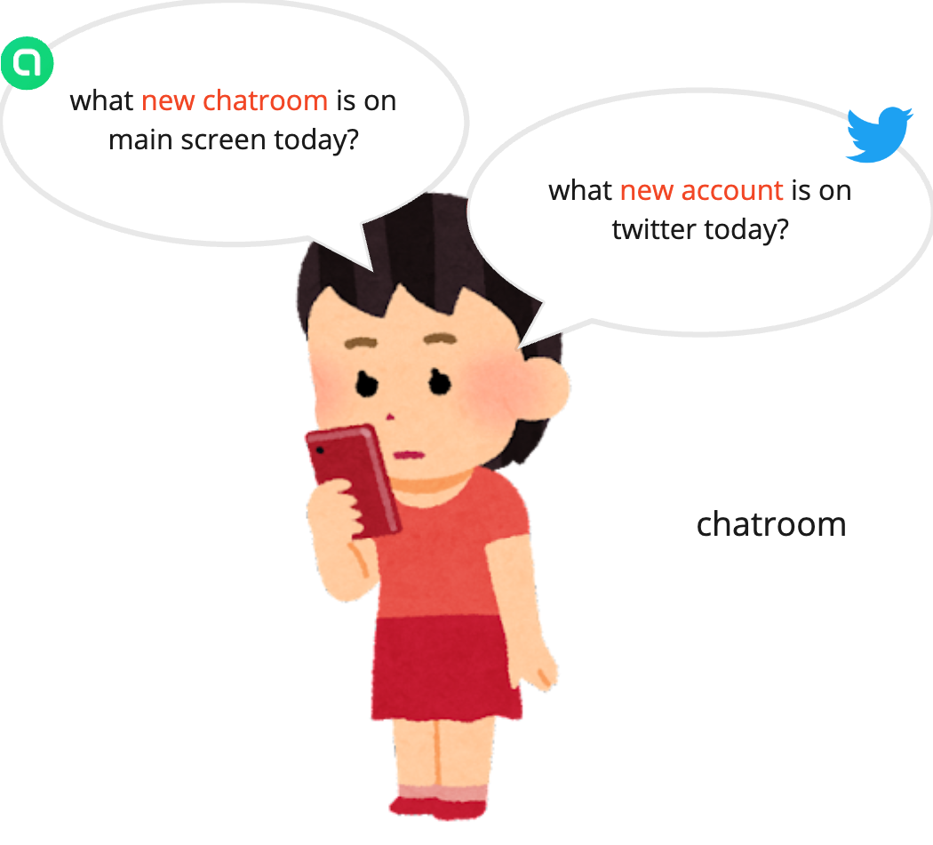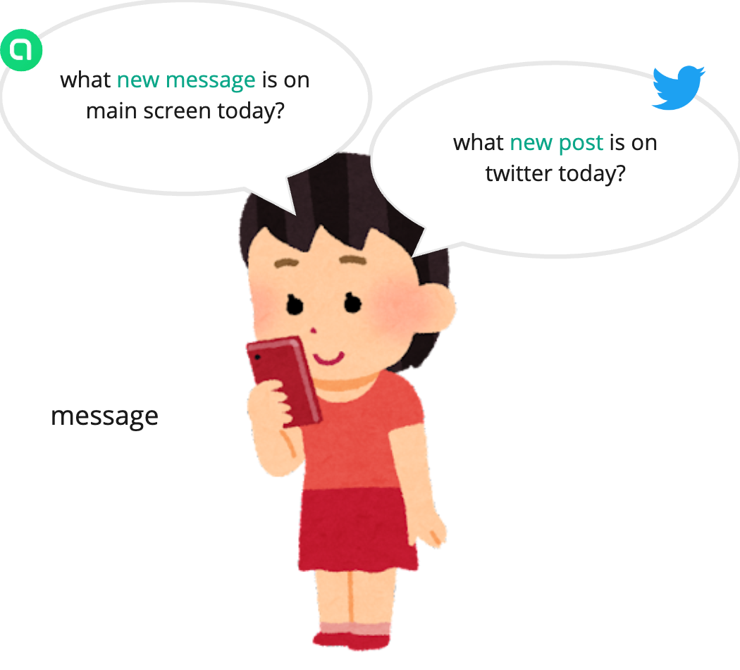However, unlike microblog posts, individual messages in most OpenChat chatrooms aren't suitable as stand-alone pieces of content. Due to the nature of mobile chats that are quickly exchanged, there are many typos and incomplete sentences. Isolating one message from a chat often makes it hard to grasp the full context.

Thus, we decided to group messages of similar topics into content, using main keywords within messages to reveal the topics more visibly. The core of this approach is extracting trending topic keywords from message text corpora. I'll explain how we implemented and applied this method.

Frequency-based trending keyword selection

First, let's look into the criteria and method by which we identified current trending keywords in message text data.

Trending keyword detection

To detect trending keywords, you might think of simply picking words with high recent occurrence frequency. But applying this to OpenChat might lead to the selection of everyday terms like greetings and expressions of gratitude or laughter rather than timely topic-specific words. This is because OpenChat communities are spaces where users regularly engage in casual chats, and new members frequently join, making greetings, introductions, and welcome messages have a significant presence.

Therefore, we decided to define trending keywords as words whose frequency has increased substantially, measured by day-to-day word frequency. The aggregation window was one day for two reasons: first, to secure a statistically significant sample size. Second, because data analysis showed that most users only visit the OpenChat main screen once a day.

When measuring increases in frequency, we set the frequency from a week ago for that word as the baseline. This method has two advantages: the first being that when a particular subject becomes a hot topic, its popularity often doesn't fade away in just one day, and considering only the difference from the previous day might lead to a situation where the word is not detected as trending due to slight changes, even if it's at the peak of popularity, which is discussed further with an example below. The second benefit is that this approach naturally filters out words related to days of the week that are mentioned repeatedly on a weekly basis. We even designed it to compare frequencies from a month earlier, though we'll skip that for brevity.

We used the Z-test statistic for the two-sample difference of proportions test (reference), to quantify the difference between two frequency values. For each word, we calculate the Z-test statistic and use that score to choose trending keywords with high scores. Although verifying a hypothesis based on p-value isn't precise since individual messages may not be independently written, a minimum trending score threshold can be set intuitively based on the normal distribution curve. Another advantage is that the noise effect, which becomes more pronounced when the frequency is low, can be accounted for based on the theory of statistical inference.

Symbols used in formulas for reviewing the Z statistic are defined as follows:

• $f_i$: frequency of the target word (term frequency, TF); the number of messages that include the word, with $i = 1$ for current TF and $i = 0$ for previous baseline TF
• $M_i$: total number of messages on the date
• $\hat{p}_i = f_i / M_i$
• $\hat{p} = (f_0 + f_1) / (M_0 + M_1)$

With these definitions, the Z statistic is as follows:

$Z={\Large \frac{(\hat{p}_1 - \hat{p}_0)}{\sqrt{\hat{p}(1-\hat{p})(\frac{1}{M_1}+\frac{1}{M_0})}}}$

One point to note is that there is a propensity for the Z value to be larger despite only minor differences in proportion as frequencies grow. Considering this, we targeted only words that have increased in frequency by at least 30%.

The graph below demonstrates how the Z values change using different baseline days for the keyword "梅雨入り" (start of the rainy season) during a week when Japan's rainy season began. The baselines compared are a day ago (blue line), two days ago (yellow line), three days ago (green line), and a week ago (red line). All data analysis involved only publicly available OpenChat messages.

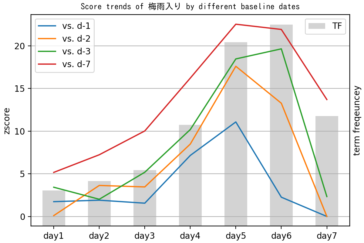
In the graph, when the baseline is one day ago (blue line), you can see a sharp decline in Z values on day 6, even though the frequency continues to rise. Importantly, on day 7, although frequency remains higher than on day 4, the Z values drop significantly below 3 except in the case of the one-week baseline (red line).

The table below illustrates how top keyword rankings are selected on day 6, depending on different baselines. When comparing three days or a week ago, the keyword '梅雨入り' is spotted as the trendiest, but it doesn't even chart in the top 10 with the one-day-ago baseline. Also, using the one-week-ago baseline setting excludes words like '今週末' (this weekend) and '今週' (this week) from being identified.

Rank	vs. d-1	vs. d-2	vs. d-3	vs. d-7
1	大雨	大雨	梅雨入り	梅雨入り
2	宝箱	梅雨入り	大雨	梅雨
3	雨降り	梅雨	梅雨	金魚
4	インドネシア	線状降水帯	線状降水帯	大雨
5	梅雨	雨降り	雨降り	線状降水帯
6	足元	土砂降り	今週末	満月
7	台風	利確	今週	九州
8	満月	今週末	土砂降り	インドネシア
9	阪神	満月	満月	cpi
10	湿気	メール	小雨	梅雨明け

MinHash-based message deduplication

Recommending a set of messages where the texts are almost identical could make users feel like they're receiving redundant information. If each message were written independently, the chance of texts overlapping would be slim. However, in reality, identical texts often occur due to actions like copy-pasting. Therefore, we need to remove texts that are nearly duplicates before aggregating frequencies to achieve the intention of extracting trending keywords.

We adopted a MinHash-based clustering method. It can efficiently apply to large data while covering cases where most text overlaps, not limited to when the strings are completely identical. Simply put, MinHash is a dimensionality reduction technique. It represents the document in a set of words and converts it into integer values, selecting the minimum of hashed function values, hence the term "MinHash".

MinHash's excellent property is that the probability of two sets sharing the same MinHash value equals their Jaccard similarity. By obtaining k independent MinHash values and using these as signatures, known as k-MinHash signatures, you can approach the match rate among document signatures as an approximate similarity.

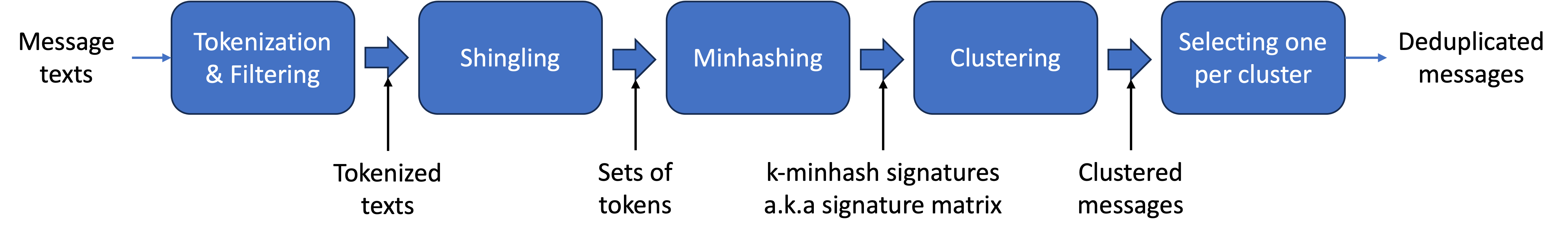
Here's how we applied it:

1. First, tokenize the text and mechanically filter only the significant tokens. We retained mainly nouns.
2. Each message is represented as a set of remaining tokens. This process is called "shingling", and an element of this set is known as a "shingle". To increase accuracy, you can compose the shingle unit with n-gram tokens.
3. Then, compute a MinHash signature, size k, for each message.
4. Group messages with the same signature into a single cluster. While it's possible to use distance-based clustering with signature match rates as similarities, our issue was that having some messages misremoved or unremoved didn't lead to significant impacts, so we chose a simpler method.
5. In each cluster, retain only one message, categorizing the rest as duplicates, and eliminate them.

When k is large, only fully identical texts are assigned to the same cluster. As k lowers, texts with less overlap also group together. To find a k value suitable for deduplication, we use a similarity metric for messages within a cluster. Existing general clustering evaluation metrics compute similarities for every pair of instances, leading to a high computational load. Instead, we defined a diversity metric that calculates for sets $\{S_i\}$ in a cluster with linear time complexity:

$\mathrm{SetDiv}(\{S_i\}):={\LARGE \frac{|\cup_i{S_i}|-|\cap_i{S_i}|}{\sum_i{|S_i|}}}$

This metric equals 1 when $|\cap_i{S_i}|=0$ and $|\cup_i{S_i}| = \sum_i{|S_i|}$ meaning there are no common elements among any two sets; conversely, if $|\cup_i{S_i}| = |\cap_i{S_i}|$, where all sets are identical, it becomes 0. When $\mathrm{SetDiv}(\{S_i\}) = p \in (0, 1)$, the influence of the intersection size term decreases as the number of sets increases, it can be approximated as $\mathrm{SetDiv}(\{S_i\}) \approx |\cup_i{S_i}| / \sum_i{|S_i|}$. As a result, $p$ proportion can be considered to consist of unique elements that don't appear in other sets and are only present once.

Naturally, we define the overlap degree as $\mathrm{SetDup} := 1-\mathrm{SetDiv}$. Finally, calculate the average overlap degrees of all clusters to measure overall clustering quality.

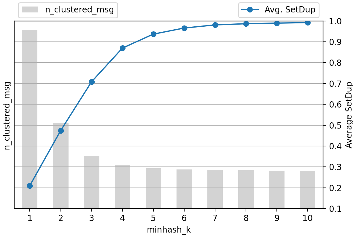
The overlap degree defined represents precision. Alongside, we compare the detected number of duplicate messages, or those grouped into clusters of size 2 or more, to choose a k value.

The following graph compares the quality of MinHash clustering with varying k values. As k increases, the overlap degree rises while the detected amount of duplicate messages drops. Believing texts over 90% overlapping can be considered duplicates, we settled on k as 5.

The following samples are from clusters with numerous messages. Top clusters exhibited overlap degrees nearing 1, essentially composed of identical texts. Common keywords in clusters include 'paypay', 'temu', 'shein', 'tiktok', '無料' (free), '招待' (invitation), and 'ギフト' (gift), suggesting topics related to marketing events for external services. With MinHash-based message duplication removal, unsuitable keywords can be controlled and prevented from being extracted as trending.

Cluster size	SetDup	Common words
3836	99.95%	[ため, 招待, 分, 最大, タップ, ポイント, paypay, temu]
1474	99.89%	[追加, 招待, 無料, get, 公式, 協力, ギフト, アカウント, temu]
1112	99.39%	[ステップ, 招待, 活動, 一流, フリーギフト, ギフト, temu]
1087	99.95%	[shein, 招待, 無料, よう, アプリ, 獲得, 手, 入手, ギフト]
576	99.05%	[報酬, 今, 参加, lite, tiktok, get]
519	99.97%	[報酬, スター, 一緒, lite, tiktok, get]
486	100.00%	[報酬, pr, tiktok, get, ログイン, 一緒, お友達, lite]
301	99.64%	[天魔, 孤城, 園, 空中庭園, モンスト, 人達同士, マルチ, マルチプレイ, 一緒, タップ, url]
296	99.72%	[おやつ, 猫ちゃん, ため, 無料, 下, 手, 猫, 獲得, リンク, ギフト, タップ]
296	99.93%	[shein, あと, プレゼント, 招待, 無料, クリック, 今, 手, 前]

Co-occurrence frequency-based keyword quality enhancement

The trending keyword scoring formula introduced earlier considered keyword frequency independently. But the context in which a word is mentioned is also valuable. Let's talk about ways to boost trending keyword quality by using co-occurrence frequency with other words as context information.

NPMI-based improper keyword filter

The OpenChat main page is accessible to people of all ages. Given this, while some keywords do reflect the trends of the OpenChat community, they're not suitable for exposure to minors. Examples include keywords tied to betting on race events such as horse racing, boat racing, cycling, and similar activities.

Initially, we created a blacklist of related keywords so that words matching these or containing them as substrings wouldn't be identified as trending keywords. However, this approach missed unexpected words, such as names of provincial cities where races are rarely held, or names of horses, jockeys, or teams that aren't practical to predefine, which ended up being extracted as recommended keywords.

To tackle this, a data-driven statistical approach was necessary. So, we introduced a keyword set expansion based on co-occurrence frequency. Here's how this method works.

We first set a small seed keyword set. Empirically, using just five words related to racing tracks ("競馬", "競艇", "競輪", "レース", "馬券") was adequate. Keeping the seed set minimal helps manage it efficiently and avoid excessive detections. Next, for candidate trending keywords, we calculate the association score based on co-occurrence frequency with each seed word. If any association score exceeds a pre-defined threshold for any seed word, we exclude that candidate word from being a trending keyword.

We used normalized pointwise mutual information (NPMI) as the association metric. To explore PMI and NPMI forms, let's define symbols:

• $f_x, f_y$: occurrences of words x and y, respectively
• $f_{xy}$: joint occurrences of words x and y
• $M$: total number of messages
• $p_x, p_y, p_{xy}$: $\small f_x / M, f_y / M, f_{xy} / M$

With these definitions, PMI and NPMI values are:

• $\mathrm{pmi}(x;y) := \log_2{\Large {\frac{p_{xy}}{p_x p_y}}}$
• $\mathrm{npmi}(x; y) := {\Large -\frac{\mathrm{pmi}(x; y)}{\log_2{p_{xy}}}}$

The NPMI metric limits its range between -1 and 1, meaning that if the occurrence probabilities are independent, it yields 0. A positive value indicates frequent co-occurrence, while a negative value suggests the opposite. Thus, you can intuitively interpret the values.

Below are words observed to have high NPMI values with the previously mentioned seed words:

Word	Seed	NPMI	Word	Seed	NPMI	Word	Seed	NPMI
あーちゃん	競艇	0.841	ワイド	レース	0.476	コース	レース	0.315
note	競艇	0.684	耐久	レース	0.465	決勝	レース	0.315
狙い馬	レース	0.647	11r	レース	0.452	イン	レース	0.308
好勝負	レース	0.636	直線	レース	0.445	最終	レース	0.304
注目馬	レース	0.636	京都	レース	0.424	パワー	レース	0.303
連単	馬券	0.627	f1	レース	0.423	スタート	レース	0.296
単穴	レース	0.619	丸亀	レース	0.407	期待	レース	0.286
穴馬	レース	0.609	ノート	競艇	0.402	スピード	レース	0.285
近走	レース	0.592	富士	レース	0.402	上位	レース	0.284
未勝利	レース	0.590	予想	競馬	0.393	東京	レース	0.280
騎手	レース	0.567	出来	レース	0.391	ペース	レース	0.280
前走	レース	0.566	予選	レース	0.377	タイム	レース	0.270
発走	レース	0.561	ご用意	レース	0.368	スーパー	レース	0.252
回収率	レース	0.547	先週	競馬	0.368	参戦	レース	0.245
馬場	レース	0.546	天候	レース	0.367	プラス	レース	0.239
ダービー	馬券	0.543	有利	レース	0.355	更新	レース	0.239
24h	レース	0.529	本線	レース	0.352	大会	レース	0.228
馬連	レース	0.508	展開	レース	0.348	結果	レース	0.227
勝負	レース	0.491	狙い	レース	0.325	アップ	レース	0.225
的中	レース	0.483	ベスト	レース	0.325	日本	競馬	0.224

Looking at the sample, in the segment with NPMI > 0.5, there were many words containing "馬" (horse), indicating keywords likely to capture interest in race-related settings. Conversely, in the NPMI < 0.3 segment, words like "東京" (Tokyo), "日本" (Japan), often mentioned locale names, or common phrases like "期待" (expectation), "大会" (tournament), "結果" (result), and so on showed up. In the 0.3 < NPMI < 0.5 segment, terms related to competition frequently appeared, such as "勝負" (match), "予選" (preliminary), "有利" (advantage), applicable outside race-betting contexts too. After the review, it's reasonable to exclude words from this segment as trending keywords since they're not particularly enticing, besides mitigating risk. Thus, we decided on 0.3 as the threshold.

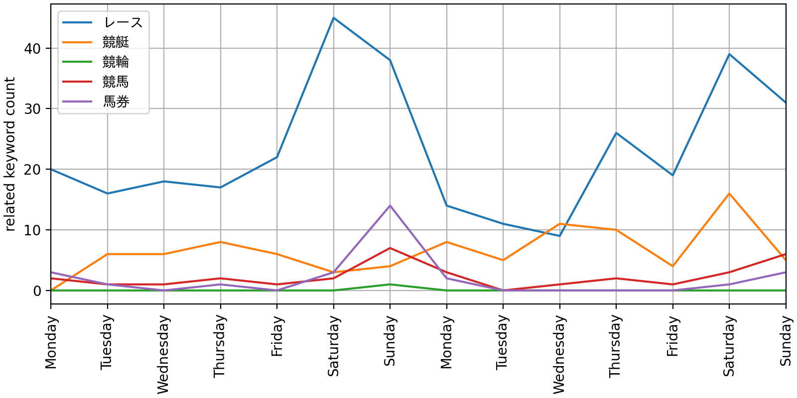
The following graph displays changes in the count of detected related keywords per seed word across two weeks. When a keyword was associated with multiple seed words, it was classified to the one with the highest NPMI value. The graph showed that many detections happened over weekends when races typically occur more often.

Diversifying top keywords using the MMR method

As previously noted, just like we avoid recommending redundant messages, it's undesirable to showcase too similar words as trending keywords altogether. The purpose of extracting trending keywords is to present related message bundles, but if different keywords lead to identical content, users could lose interest quickly. Therefore, we need to ensure words with high co-occurrence frequency aren't selected at the same time.

This is similar to the diversification problem of hashtag recommendations I introduced in a previous post using the maximal marginal relevance (MMR) method, which can be similarly applied here. As a reminder, the MMR approach selects items one by one in order of scores but considers a penalty term for similarity with previously selected items to create diverse results.

To express this in formula terms, let's define the symbols:

• $score_i$: the original trend score for keyword i, using the logarithm of the Z statistic as the score
• $\alpha$: penalty weight parameter
• $sim(i, j)$: similarity between keywords i and j
• $S$: the entire set of trend keywords for re-ranking
• $R_k$: collection of trend keywords chosen up to the k-th step

With these symbols, keyword ranked k+1 is chosen based on the largest adjusted score:

$\large score_{i} - \alpha \cdot \max_{j \in R_k}{sim(i, j)},\quad i \in S \setminus R_k$

We adopted the previously introduced NPMI metric as the keyword similarity. Besides soft constraint through the penalty term, a hard constraint was added to prevent further selection if a highly similar keyword with an NPMI value above a certain level was already chosen in an earlier step.

Here's a sample result of applying the diversification method with different $\alpha$ values:

Rank	Original list	$\alpha=0.5$	$\alpha=1.$	$\alpha=2.$	$\alpha=5.$
1	イラン	イラン	イラン	イラン	イラン
2	イスラエル	大雨	大雨	大雨	大雨
3	大雨	土砂降り	土砂降り	土砂降り	土砂降り
4	予報	雨予報	雨予報	雨予報	雨予報
5	土砂降り	雨降り	雨降り	雨降り	雨降り
6	雨予報	予報	one	one	one
7	雨降り	one	湿度	湿度	湿度
8	中止	函館	予報	函館	函館
9	小雨	中止	函館	イオン	イオン
10	one	小雨	イオン	釣り	釣り

In the initial list, 'イラン' (Iran) and 'イスラエル' (Israel) were ranked 1st and 2nd, respectively. After applying diversification, only 'イラン', the top keyword, was left given the NPMI value between them exceeding the threshold. '予報' (forecast) and '中止' (cancellation) were reasonably related to '大雨' (heavy rain), causing them to fall in rank as $\alpha$ increased. Empirical results showed consistent ranking order beyond a penalty weight of 2, leading to the decision that $\alpha$ should be set above this for fostering adequate diversity.

For reference, the example includes '土砂降り' (landslide, downpour), '雨予報' (rain forecast), '雨降り' (rainfall) in survived keywords post-diversification due to their mutual NPMI values being less than 0.3, indicating only relatively low co-occurrence in messages.

Conclusion

This article introduced methods for extracting trending keywords from OpenChat message data using statistical techniques. We spotted trending keywords as those whose frequency significantly increased based on the test statistics. Enhancements included removing duplicate messages through text clustering, eliminating inappropriate keywords based on co-occurrence frequencies, and diversifying top keywords for improved quality. Future prospects include generating trending reports based on extracted keywords using large language models (LLMs) or pursuing synergistic connections to other related services.

Above all, with users at the forefront, we'll work to ensure they discover many engaging and valuable contents in the OpenChat service, promoting active engagement. Thank you for reading to the end.