Measuring voice quality in the LINE app

The LINE app offers real-time communication services such as LINE one-on-one calls, LINE group calls, and LINE meetings, which transmit audio and video data in real time over the internet. This allows users to conveniently experience audio and video calls from anywhere.

The core challenge of real-time communication services is to simultaneously maintain real-time performance and good quality. To identify and improve any inconveniences or problems users may experience while using the service, objective and fair quality measurement and evaluation are essential. In this article, we'll first look at how we measure quality, and then explore three representative areas of quality measurement: acoustic echo cancellation (AEC), frequency response, and loss robustness.

Aspects of quality measurement

We recognize the importance of service quality and thoroughly measure it in the following various aspects:

Response to acoustic environments

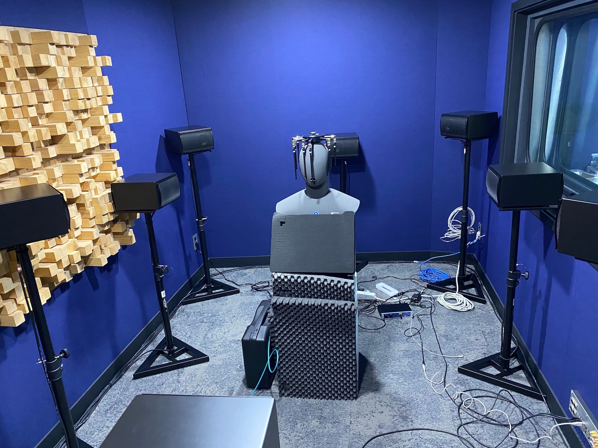
The acoustic environment refers to the acoustics around the person making the call. The spatial characteristics of the caller can influence the call quality. For example, if the surroundings are noisy or echoey, the call quality can deteriorate, causing discomfort. We aim to evaluate the performance of voice processing technology in such acoustic environments and derive technical improvements. To do this, we have set up an anechoic chamber and are measuring acoustic variables that affect the performance of voice processing technology.

Firstly, please refer to the article titled Technology to Improve Voice Quality During Video Conferences (available in Korean only) published on the former LINE Engineering blog, which explains how to set up a caller's environment to improve voice quality.

Acoustic variables in the acoustic environment include background noise, volume level, reverberation level, and echo. We quantify these acoustic variables by dividing them according to their characteristics. For example, for background noise, we quantify how much ambient noise is removed, and for echo, we quantify how much echo is removed.

We also have an anechoic chamber environment to measure these acoustic variables. In an anechoic chamber environment, we can simulate various acoustic variables to closely reproduce the actual environment and measure whether the voice processing technology we use internally operates appropriately. For example, to simulate a call environment in a cafe, we play background noise recorded in a cafe and measure the impact of this noise on voice quality.

Response to network environment changes

Changes such as packet loss, packet delay, bandwidth throttling, and network congestion continuously occur in the network, and these changes in the network environment have a significant impact on the quality of real-time call services. Therefore, to ensure that users consistently experience excellent service quality, it's necessary to measure the impact of network environment changes on service quality and develop technologies and strategies to maintain good quality. For this, we first need technology to accurately analyze and diagnose network environment changes in real time, and based on the diagnostic results, we need to implement various strategies such as bitrate adjustment and data retransmission to maintain service quality. Measuring these technologies and strategies quantitatively is very important as they have a direct impact on the quality perceived by users.

In reality, network environment changes occur in various forms. We model these changes according to different situations, create various scenarios, and apply each scenario to a simulation to simulate network environment changes in real life. Then, we quantitatively measure the quality (in terms of voice quality, video quality, frames per second, data usage, and so on) at that time to evaluate whether the network environment changes and response strategies are working effectively.

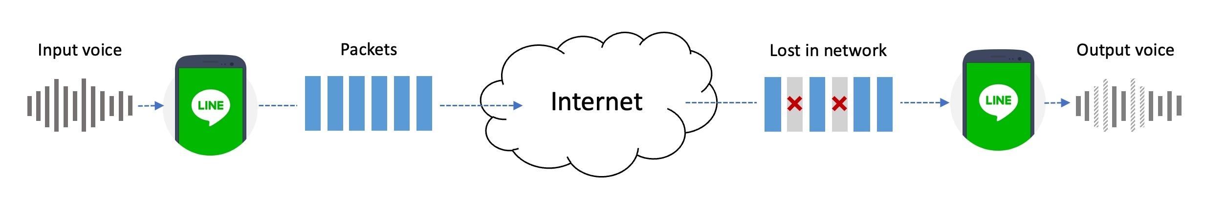
The following image is an example of a simulation that reproduces a scenario modeled on packet loss occurring in a real environment.

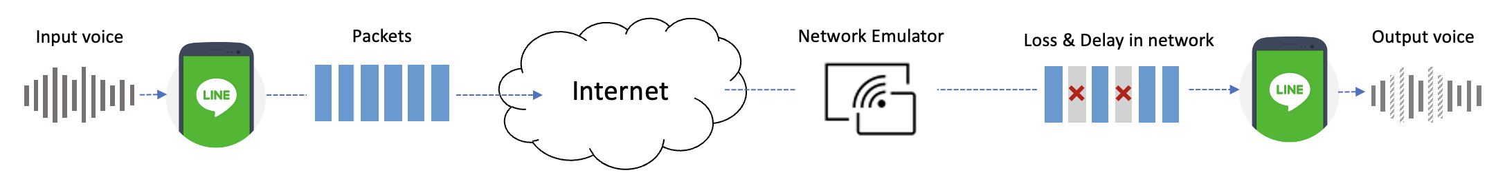
As in the example above, we use a network emulator to induce packet loss, reproduce the actual environment, and quantitatively measure the degradation of sound quality due to packet loss. In addition to packet loss, the network emulator can simulate network environment changes such as packet delay and bandwidth throttling, and by connecting multiple network emulators, it can simulate various network environment changes simultaneously.

Through these simulations, we quantitatively measure the quality in each environment by simulating various network environment changes, and by repeating these measurements, we evaluate the reliability of the technology and derive improvements.

Response to global environments

The LINE app is a global service used all over the world. Therefore, it's very important to consistently provide excellent quality to global users. However, each region's communication network and infrastructure use various internet service providers (ISP), network topologies, bandwidth allocations, network environments, and management methods. In addition, Wi-Fi infrastructure, usage patterns, and culture can vary, and the network environment can change depending on factors such as whether calls were made during the weekdays or weekends, or during regional events.

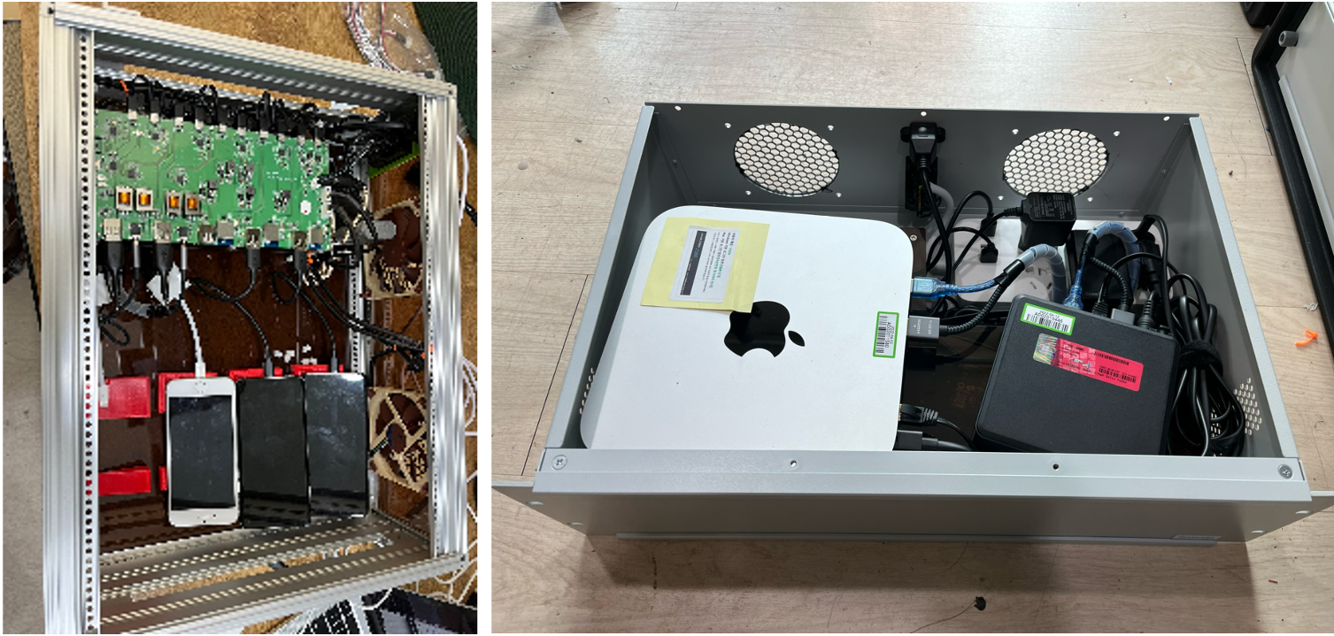
To respond to these regional differences and environmental changes, we have deployed our self-developed quality measurement tool in about 15 countries worldwide and continuously monitor the network environment characteristics of each country. Through this, we understand the network characteristics and changes of each country and region, apply the optimal settings, and provide the best service quality to users.

The measurement tool equipped with our self-developed quality measurement H/W and S/W automatically makes calls and measures various quality metrics such as voice and video quality, delay, and call connection time. When measuring quality, we use not only international standard measurement metrics such as POLQA (ITU-T P.863) and PSNR (ITU-T J.340), but also measurement metrics that aren't standard but widely used in the industry.

  

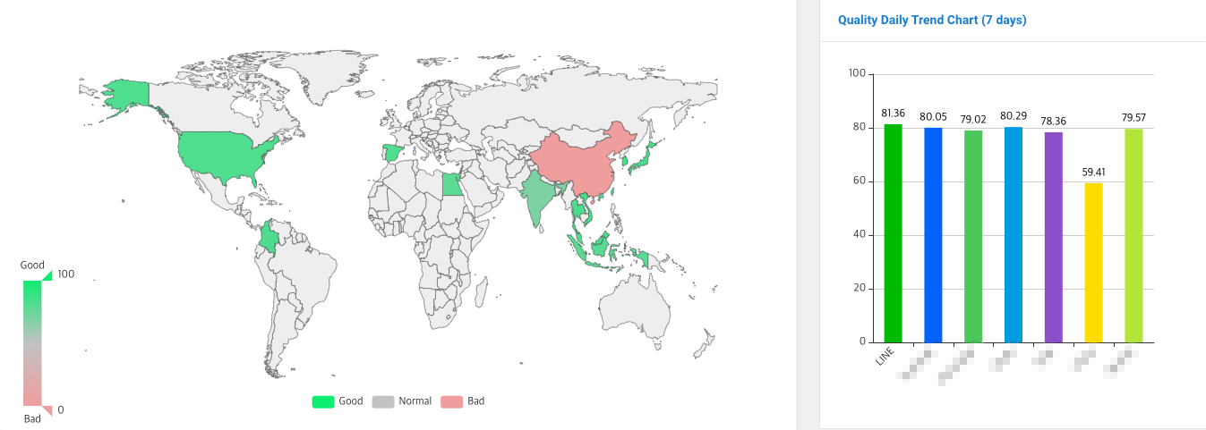
Through such global quality monitoring, we compare and analyze our quality with other services to identify our strengths and areas for improvement. The global monitoring system aggregates the metrics measured by the quality measurement tool and expresses them as a comprehensive service quality evaluation score. The service quality evaluation score is distinguished by different colors as shown below, making it easy to understand the quality level by region. In the map below, green represents areas where the quality is smooth, gray represents areas where the quality is average, and red represents areas where the quality isn't good or measurement isn't possible.

We are constantly studying and implementing measures to improve quality, taking into account the unique network and environment of each country and region, and we are continually striving to provide the best service quality in all regions.

External testing

We also carry out independent measurements through external testing. External testing is an important process where third-party experts measure the performance of our product and quantitatively analyze voice and video quality.

In the external testing process, we coordinate the measurement scenarios with the external testing company to accurately grasp the quality changes in the testing environment. Furthermore, the process includes comparing performance with other services to evaluate product competitiveness in the market. Through this, we accept quality evaluations from a neutral perspective and derive improvements to enhance user satisfaction.

Measuring AEC performance

AEC is a technology that suppresses acoustic echo in a voice call system, reducing instances of the user's voice being heard again as an echo after passing through the other party's microphone. The image below illustrates an example of echo occurring in a voice call system.

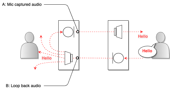
In the image above, when the sound (B) from the user on the right is output through the speaker of the user on the left, that sound is also collected by the microphone (A). An echo refers to the sound reflecting off a medium and coming back. The microphone that transmits the collected sound can be considered the major source of reflection. If the user's voice is collected from the other party's microphone and directly transmitted back to the user, the user will hear their voice again after a short delay. The call AEC detects this acoustic echo in real time and appropriately filters and removes it to improve voice call quality.

We are developing AEC with our own technology and introducing machine learning technology to provide high-quality echo removal performance. Through this, we measure the quality so that LINE app users can enjoy voice calls with clean and high sound quality without the discomfort caused by echos. Before we go into detail about how we measure, let's define the terms used in AEC performance measurement and performance metric description.

• Near-end: Refers to the user located on the side where the measurement is taking place in the call system.
• Far-end: Refers to the user who is on a call with the near-end.
• Single talk: Refers to when only the near-end or far-end is speaking.
• Double talk: Refers to when both the near-end and far-end are speaking.

Method of measuring AEC performance

AEC performance is evaluated by quantifying the ability to suppress echo without degrading the audio, and the following procedure is followed when measuring performance.

Setting up the measurement environment

First, we set up the measurement system environment for measuring AEC performance.

Selecting a quality measurement tool

We use AECMOS to evaluate and improve AEC performance. AECMOS is a tool that measures the ability to suppress echo without degrading the audio through objective metrics. It's currently used in the industry and academia to evaluate AEC performance. It's used to evaluate the performance of new algorithms, compare with existing technologies, or analyze experimental results in research papers or reports and compare with other research to prove the validity of the research.

AECMOS has the following three measurement modes:

• 48,000 Hz, scenario-based model (Run_1668423760_Stage_0.onnx)
• 16 kHz, scenario-based model (Run_1663915512_Stage_0.onnx)
• 16 kHz model (Run_1663829550_Stage_0.onnx)

The scenario-based model can produce more accurate results as it knows the ST FE (far-end single talk), ST NE (near-end single talk), and DT (double talk) section information. We use the 48,000 Hz, scenario-based model for AEC performance measurement.

AECMOS has four sub-metrics as follows (for more details, refer to the Meaning of performance metrics section).

Metric	Explanation
ST FE Echo DMOS	Quality of echo removal in far-end single talk
ST NE MOS	Quality of voice preservation in near-end single talk
DT Echo DMOS	Quality of echo removal in double talk
DT Other MOS	Quality of voice preservation in double talk

Selecting a test data set

For the test data set, we use the test_set_icassp2022 data set provided by the AEC challenge. This data set provides 300 DT cases, 300 ST FE cases, and 200 ST NE cases of sound sources.

Preparing the measurement target module

Prepare the AEC module that will be the target of performance measurement.

Measuring AEC performance

Once the measurement environment is set up, AEC performance is measured following these steps:

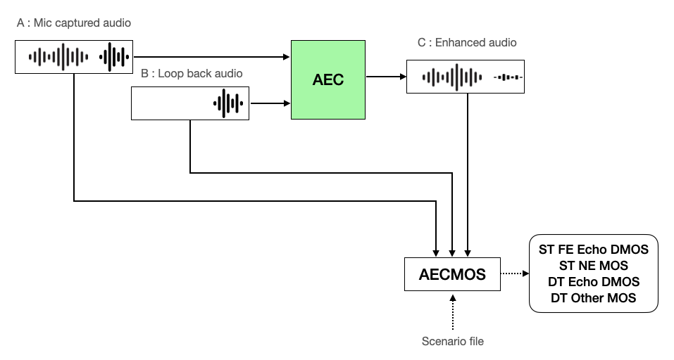
1. Input A (the original voice mixed with echo, referred to as "mic captured audio" in AECMOS) and B (the voice that is the source of the echo, referred to as "loop back audio" in AECMOS) into the AEC.
2. Input the scenario file, the AEC processing result C (the voice with the echo removed, referred to as "Enhanced audio" in AECMOS), and A and B into the AECMOS measurement tool to measure ST FE Echo DMOS, ST NE MOS, DT Echo DMOS, and DT Other MOS.

Evaluating AEC performance

We analyze the results of the AEC performance measurement to see where differences have occurred, what has improved, and what is lacking, then we establish future development and update plans based on this.

Meaning of AECMOS metrics and comparison of perceived quality by metric

Let's look at the meaning of the metrics measured by AECMOS and compare the perceived quality for each metric score. For convenience's sake, we will assume that the near-end is "me" in the explanation.

Meaning of performance metrics

As mentioned before, AECMOS has four metrics, each with the following meaning:

• ST FE Echo DMOS: A measure of the amount of echo remaining after echo removal in an environment with only echo (an environment where only far-end's voice is in A). It's expressed as a score between 1 and 5, with higher numbers indicating better echo removal.
• ST NE MOS: A measure of the quality of my preserved voice in an environment where only the near-end's voice is present and there is no echo (an environment where only the near-end's voice is in A, the presence of B's voice isn't important). It's expressed as a score between 1 and 5, with higher numbers indicating better voice quality.
• DT Echo DMOS: A measure of the quality of the remaining echo after echo removal in a double talk environment (an environment where near-end and far-end voices are both in A). It's expressed as a score between 1 and 5, with higher numbers indicating better echo removal.
• DT Other MOS: A measure of the quality of the preserved voice after echo removal in a double talk environment (an environment where near-end and far-end voices are both in A). It's expressed as a score between 1 and 5, with higher numbers indicating better voice quality.

To achieve the best call quality, all scores should be high. However, in reality, it's almost impossible to accurately distinguish only the echo signal, so voice degradation also occurs during the echo removal process. Especially in the double talk section where echo and voice exist at the same time, the two voices mix, so the possibility of voice degradation during echo removal is higher. Because of this, echo removal and voice preservation are in a trade-off relationship.

ST FE Echo DMOS and DT Echo DMOS scores increase as echo is better removed, and ST NE MOS and DT Other MOS scores increase as voice is better preserved. Therefore, if all sounds are removed for high ST FE Echo DMOS and DT Echo DMOS scores, both echo and voice can be removed for high scores, but the other party can't hear my voice properly. Conversely, if signals aren't removed for high ST NE MOS and DT Other MOS scores, my voice remains intact for high scores, but the conversation is difficult because of the severe echo.

Comparison of perceived quality by AECMOS performance metrics

In the table below, you can perceive the difference in voice quality according to the score ranges of the four quality metrics of AECMOS: ST FE Echo DMOS, ST NE MOS, DT Echo DMOS, and DT Other MOS.

ST FE Echo DMOS	Audio Capture Location	Audio File	Description
Original	Mic captured audio (A)		The person at the far end (far-end) speaks alone (B), and this sound is collected (A) by my microphone as it's output through my speaker. You can hear an echo at A.
	Loop back audio (B)
1.x	Enhanced audio (C)		The echo wasn't well removed.
2.x	Enhanced audio (C)		The echo has decreased, but there are many sections where the residual echo can be heard.
3.x	Enhanced audio (C)		Overall, a lot of the echo has been removed, but you can occasionally hear some residual echo.
4.x	Enhanced audio (C)		The echo has been completely removed and can't be heard.

ST NE MOS	Audio Capture Location	Audio File	Description
Original	Mic captured audio (A)		This is a situation where a loud noise occurs from the far-end while I (near-end) am speaking in an echo-free environment. There is far-end noise at B, but at A, there is only my voice.
	Loop back audio (B)
1.x	Enhanced audio (C)		Despite being in an echo-free environment, there is significant degradation to the near-end voice. The degraded sections are unintelligible.
2.x	Enhanced audio (C)		Despite being in an echo-free environment, there is degradation to the near-end voice. You need to listen carefully to understand the degraded sections.
3.x	Enhanced audio (C)		Despite being in an echo-free environment, there is slight degradation to the near-end voice. There is degradation, but it's understandable.
4.x	Enhanced audio (C)		There are hardly any sections where the near-end voice is degraded.

DT Echo DMOS	Audio Capture Location	Audio File	Description
Original	Mic captured audio (A)		The near-end starts speaking first and the far-end speaks along (B). Both voices are collected together by my microphone (A).
	Loop back audio (B)
1.x	Enhanced audio (C)		The echo wasn't well removed.
2.x	Enhanced audio (C)		The echo has decreased, but there are many sections where the residual echo can be heard.
3.x	Enhanced audio (C)		Overall, a lot of the echo has been removed, but you can occasionally hear some residual echo.
4.x	Enhanced audio (C)		The echo has been completely removed and can't be heard. There was degradation to the near-end voice, but a high score was measured because the DT ECHO DMOS score only evaluates the amount of residual echo.

DT Other MOS	Audio Capture Location	Audio File	Description
Original	Mic captured audio (A)		The near-end starts speaking first and the far-end speaks along (B). Both voices are collected together by my microphone (A).
	Loop back audio (B)
1.x	Enhanced audio (C)		There is significant degradation to the near-end voice during the double talk section. The degraded sections are unintelligible.
2.x	Enhanced audio (C)		There is degradation to the near-end voice during the double talk section. You can only realize that someone is speaking in the degraded sections.
3.x	Enhanced audio (C)		There is slight degradation to the near-end voice during the double talk section. You need to listen carefully to understand the degraded sections.
4.x	Enhanced audio (C)		There is degradation to the near-end voice during the double talk section, but it's understandable. The amount of echo from the far-end doesn't reflect in the DT Other MOS score, but it does affect the DT Echo DMOS value.

AEC performance measurement summary

We measure performance as follows to reliably evaluate and improve our AEC technology:

• Ensuring reproducibility and consistency: We measure performance in a repeatable environment using AECMOS. We conduct tests locally using the same database to reduce network influence. Using a measurement method that delivers consistent results in the same environment allows us to accurately understand performance changes and improvements in AEC technology.
• Using reliable metrics: The AECMOS metric is a crucial metric widely used in the industry and academia for AEC performance evaluation and comparative analysis. Using this metric ensures the reliability of the measured performance, and allows us to quantitatively evaluate the product's numbers and performance and set the direction for improvement.
• Verifying performance in various echo situations: We use the following methods to quantitatively check how AEC technology works in various echo environments.
  • Large database: We use more than 2400 databases where single talk and double talk are mixed according to the scenario.
  • Diverse recording environments: We use data with various voice and echo volumes and characteristics, recorded on various audio devices (microphones, speakers) and environments.

We strive to provide the best voice quality by reliably evaluating performance under various conditions so that our AEC technology can work effectively in any echo situation.

Also, we've developed echo removal technology using machine learning to overcome performance problems arising because echo removal and voice preservation are in a trade-off relationship. As a result, the overall performance metrics have been uniformly improved compared to the existing technology. Although machine learning characteristics improve performance with more computations, we are still tuning by appropriately adjusting the amount of computation as we can't use a lot of computations in real-time call services yet (such high-performance AEC is only installed in LINE desktop).

So far, we've made many improvements. In the future, we aim to further improve performance in double talk situations and install high-performance AEC in mobile apps.

Measuring frequency response

Next, let's look at the method of measuring frequency response. First, let's briefly look at several concepts related to frequency response measurement and learn about the frequency response measurement method and procedure. 

What are frequency and sampling rate?

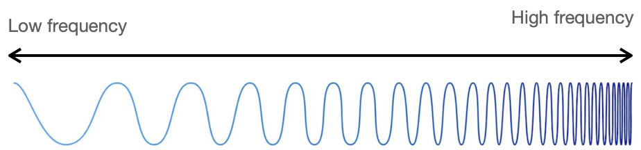
Frequency is the periodic repetition of vibrations. Frequency is typically indicated by the number of vibrations per second, and the unit used is hertz (Hz). High frequency represents vibrations that repeat quickly with a short period, while low frequency represents vibrations that repeat slowly with a long period.

Since sound is created by vibrations in air or other media, sound can also be expressed in frequency. The height of the frequency determines the pitch of the sound. Components with a high frequency have a high pitch, and components with a low frequency have a low pitch. For example, the C note on a piano has a frequency of about 261.63 Hz, and the E note has a frequency of about 329.63 Hz.

When converting an analog signal to a digital signal, a process called sampling is used. Sampling is the process of converting the original signal into a signal composed of measured values (samples) at regular intervals, and the frequency of sampling per second is called the sampling rate. One of the important concepts in digital signal processing, the Nyquist-Shannon sampling theorem, is used to determine the sampling rate required to represent a signal digitally. According to this theorem, if you set the sampling rate to more than twice the maximum frequency of the signal to be digitized, you can perfectly reproduce the original signal digitally. Simply put, to digitize an analog signal with a frequency of 20,000 Hz, you need to use a sampling rate of more than 40,000 Hz. In this way, the digitized signal will contain almost the same information as the original signal.

What is frequency response?

Frequency response is a metric that shows how accurately an audio system's output signal is transmitted across various frequency bands, and it's used to evaluate how well an audio system reproduces a wide frequency range from low to high frequency bands. It compares the input and output sound volumes by frequency band, and uses decibels (dB) as the measurement unit. Decibels are expressed on a logarithmic scale to resemble the volume of the sound perceived by the human ear. The more negative it gets, the quieter it means, and the bigger the difference in decibel values, the bigger the auditory difference humans can feel.

Measuring frequency response is an important way to evaluate the performance of an audio system. An audio system that can reproduce more accurately over a wider frequency range is considered a higher-performing audio system. This helps to reproduce music or voices more naturally and contributes to providing users with a high-quality audio experience. 

In voice calls, the voice signal of the speaker includes a wide range of frequencies from low to high pitches. If an audio system can accurately reproduce these various frequencies, the quality of the voice call will improve. Therefore, we place importance on frequency response to provide users with the best voice call experience, and we are continuously improving the frequency response of LINE app voice call services based on the results of frequency response measurements.

Audible frequency and frequency response

Audible frequency refers to the range of frequencies that can be heard by the human ear. Typically, the human ear can hear frequencies between approximately 20 Hz and 20,000 Hz. Therefore, frequency response is primarily measured within this audible frequency range.

Frequency response is generally evaluated by graphically representing the gain (change in intensity) of the output signal compared to the original signal for each frequency band. This graph visually represents the difference in gain per frequency, allowing you to see the characteristics of the system's output signal for each frequency band. Let's look at an example of measured frequency response results below.

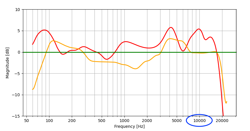
The graph above shows the frequency responses of two audio systems, represented in red and orange respectively. Here, you can easily see the difference between the ideal frequency response (green) and the red and orange frequency responses. For example, if you look at the frequency response around 10,000 Hz (marked with a blue circle), the orange frequency response is similar to the ideal frequency response, but the red frequency response is about 5 dB higher than the ideal one. Therefore, we can say that at 10,000 Hz, the orange has more ideal frequency response characteristics than the red.

Characteristics of sound by frequency band

The characteristics of sound by frequency band are as follows:

• Below 100 Hz: Classified as low frequency. Signals in this band don't help with voice calls. In fact, if the sound pressure in this part is high, it can sound uncomfortable to the listener.
• 100 Hz-250 Hz: Classified as mid-low frequency. It's mainly responsible for the bass tones and vibrations in voice calls, and plays a role in expressing the stability of the voice.
• 250 Hz-2,000 Hz: Classified as mid-frequency. This band is one of the main parts of the voice, playing a role in expressing the clarity and sharpness of the voice.
• 2,000 Hz-8,000 Hz: Classified as high frequency. The high-frequency band handles the treble part of the voice and details such as fricatives ([f], [v]).
• 8,000 Hz-20,000 Hz: Classified as ultra-high frequency. This frequency band plays a role in expressing the characteristics of sibilants ([s], [z]).
• Above 20,000 Hz: This band, where there is almost no voice signal, is difficult to perceive with human hearing.

How to measure frequency response

Frequency response is affected by all paths through which the audio signal flows. In a call system, the characteristics of the microphone and speaker devices and the call module have an impact.

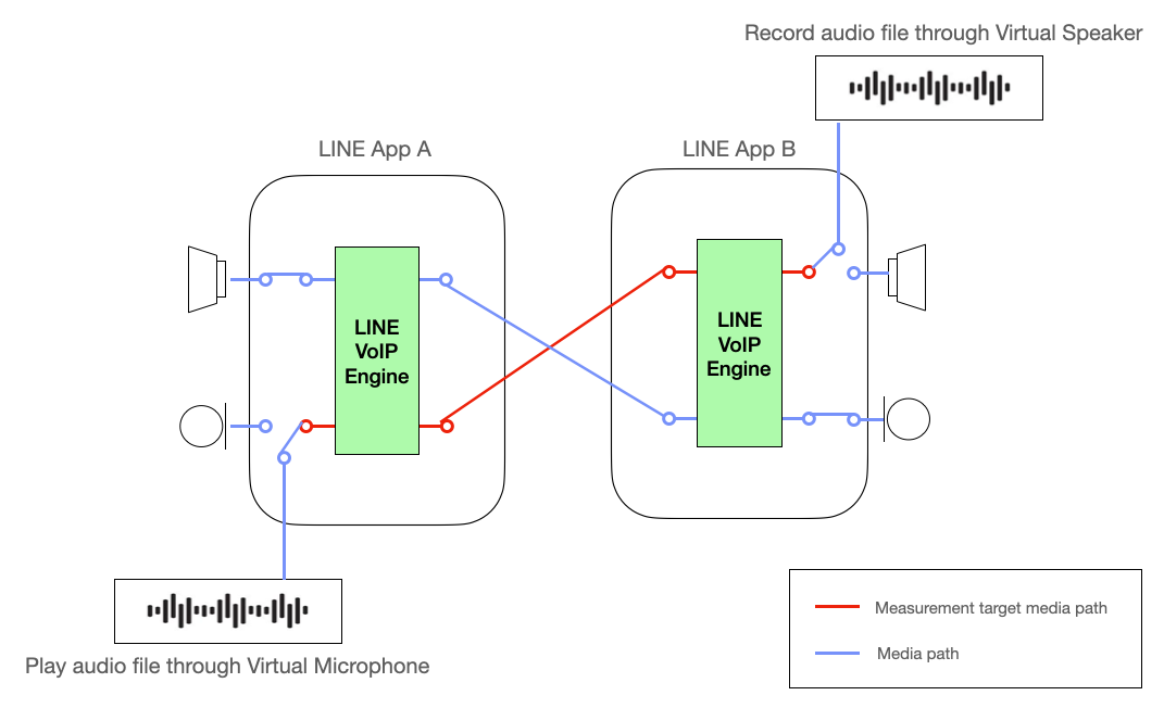
We use a virtual audio device to accurately measure the frequency response of the call module. This is to minimize the influence of the audio device during frequency measurement. The virtual audio device can input and output audio signals without distortion, allowing for accurate measurement of the characteristics of the LINE call module alone.

The red line in the image below represents the target path for measuring frequency response. By using a virtual audio device, we can exclude the influence of the audio device from the frequency response measurement results and accurately measure the characteristics of the call module alone. This allows us to effectively obtain the information needed to accurately analyze the frequency response of the call module and improve its quality.

Frequency response measurement procedure

The frequency response measurement of the LINE app call module follows the procedure below.

Selection of test signals

Select a test signal suitable for the audio system you want to measure. The frequency band of this test signal is typically composed of voice signals with signals in the audible frequency range of 20 Hz to 20,000 Hz. The reason for composing the test signal with voice signals is because the call module can mainly consider signals other than voice as noise and remove them.

The test signal uses the signal of the electrical acoustic performance evaluation standard (IEEE 269-2010) for communication devices provided by IEEE. The link below is the test signal used for such measurements.

• Download media file
  • IEEE_269-2010_Male_mono_48_kHz.wav: Initial stabilization sound source
  • IEEE_269-2010_Male_mono_48_kHz.wav, IEEE_Female_mono_48_kHz.wav: Frequency response measurement sound sources

Setting up the measurement system environment 1 - Configuring the measurement environment

Set up the system environment for measuring frequency response.

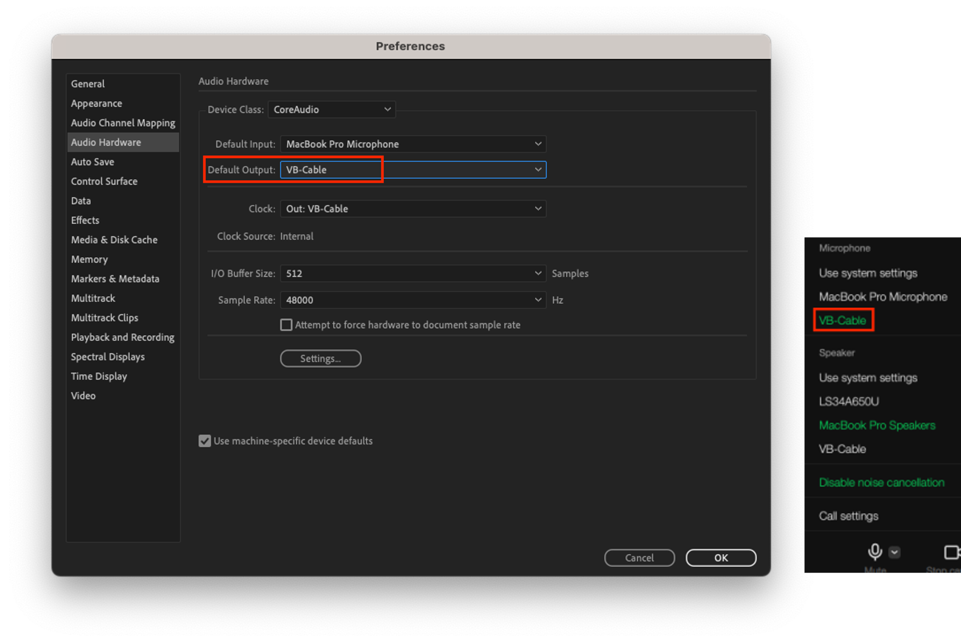
• Adobe Audition: This is a software that plays the test signal and records the output signal of the audio system being measured.
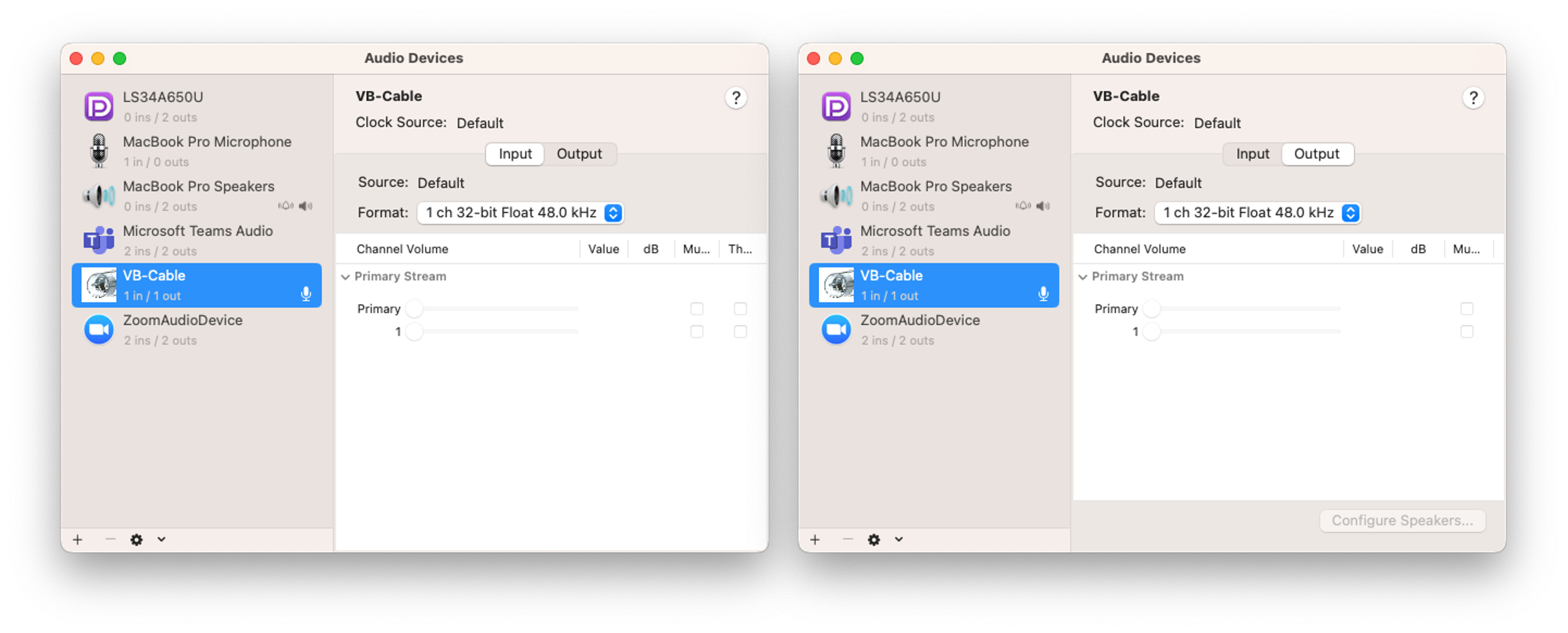
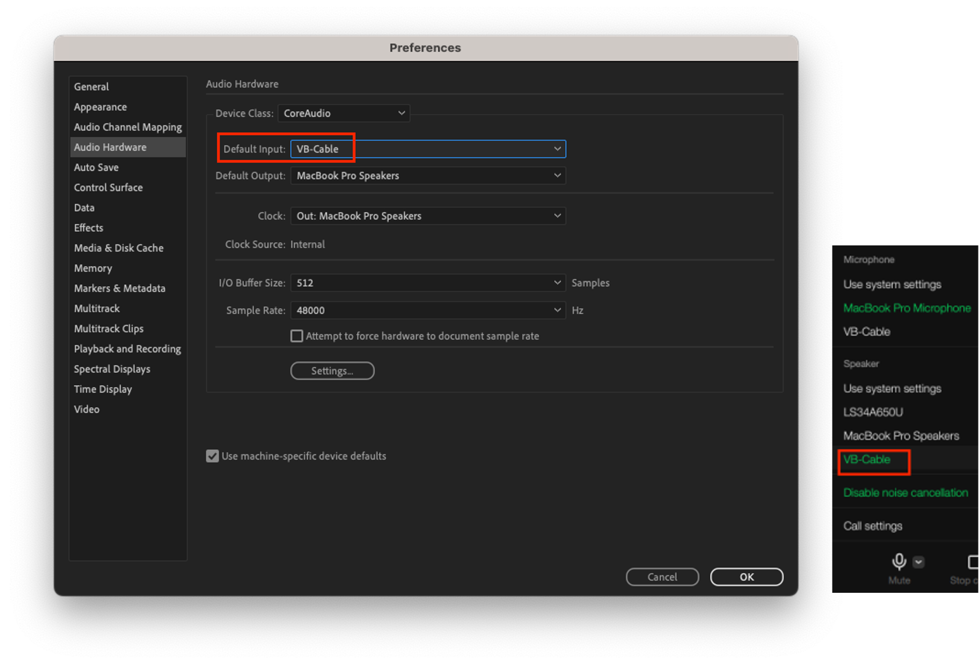
• VB-AUDIO: This is a software that allows you to use microphone input and speaker output without distorting the audio signal using a virtual audio device. After installation, you can use the VB-Cable, which is a virtual microphone/speaker device.
• Frequency response measurement tool: This is a code that takes two wav files, the measurement signal and the output signal, and draws the frequency response.
• Code that draws frequency response

  import sys
  import warnings
  import numpy as np
  import matplotlib.pyplot as plt
  import scipy.io.wavfile as wf
  from scipy.io.wavfile import WavFileWarning
  from numpy import ComplexWarning
  from scipy.interpolate import make_interp_spline
  
  # Calculate the center frequencies of 1/12 octave bands.
  def calculate_octave_bands (start_freq, end_freq):
      bands = []
      while start_freq <= end_freq:
          bands.append (start_freq)
          start_freq *= 2** (1/12) # Increase by 1/12 octave.
      return bands
  
  # Ignore the WavFileWarning
  warnings.filterwarnings ("ignore", category=WavFileWarning)
  warnings.filterwarnings ("ignore", category=ComplexWarning)
  
  if len (sys.argv) != 3:
      print ("Usage: python script.py <ref_audio_file.wav> <deg_audio_file.wav>")
      sys.exit (1)
  
  ref_fs, ref_audio_data = wf.read (sys.argv[1])  # Load the reference audio file
  deg_fs, deg_audio_data = wf.read (sys.argv[2])  # Load the degraded audio file
  
  
  # Check if sample rates are different
  if ref_fs != deg_fs:
      print ("Error: Sample rates are different. Cannot process audio files with different sample rates.")
      exit ()
  
  # Check if sample types are different
  if ref_audio_data.dtype != deg_audio_data.dtype:
      print ("Error: Sample rates are different. Cannot process audio files with different sample types.")
      exit ()
  
  # Check the audio sample type
  if ref_audio_data.dtype == np.float32:
      kMaxSample = 1.0
  else:
      kMaxSample = 32768  # For int16, 0 dBFS is 32678 with an int16 signal
  
  
  kNfft = 32768
  win = np.hamming (kNfft)
  
  num_segments = min (len (ref_audio_data), len (deg_audio_data)) // kNfft
  ref_audio = np.zeros ( (kNfft, num_segments))
  deg_audio = np.zeros ( (kNfft, num_segments))
  
  
  # Take a slice and multiply by a window
  for i in range (num_segments):
      ref_audio[:, i] = ref_audio_data[i * kNfft : (i + 1) * kNfft] * win
      deg_audio[:, i] = deg_audio_data[i * kNfft : (i + 1) * kNfft] * win
  
  # Initialize arrays to store spectral data for each frame
  num_frames = ref_audio.shape[1]
  ref_audio_sp = np.zeros ( (kNfft // 2 + 1, num_frames))
  ref_audio_s_mag = np.zeros ( (kNfft // 2 + 1, num_frames))
  deg_audio_sp = np.zeros ( (kNfft // 2 + 1, num_frames))
  deg_audio_s_mag = np.zeros ( (kNfft // 2 + 1, num_frames))
  
  # Process each frame
  for i in range (num_frames):
      ref_audio_sp[:, i] = np.fft.rfft (ref_audio[:, i])  # Calculate real FFT for each frame
      ref_audio_s_mag[:, i] = np.abs (ref_audio_sp[:, i]) * 2 / np.sum (win)  # Scale the magnitude of FFT for each frame
      deg_audio_sp[:, i] = np.fft.rfft (deg_audio[:, i])  # Calculate real FFT for each frame
      deg_audio_s_mag[:, i] = np.abs (deg_audio_sp[:, i]) * 2 / np.sum (win)  # Scale the magnitude of FFT for each frame
  
  avg_ref_audio_s_mag = np.mean (ref_audio_s_mag, axis=1)
  avg_deg_audio_s_mag = np.mean (deg_audio_s_mag, axis=1)
  
  f_axis = np.linspace (0, ref_fs/2, len (avg_ref_audio_s_mag))
  
  center_frequencies = calculate_octave_bands (60, ref_fs / 2)
  
  # Aggregate the spectral data in the frequency domain into 1/12 octave bands.
  ref_band_spectra = []
  deg_band_spectra = []
  for center_freq in center_frequencies:
      lower = center_freq / (2** (1/24))  # Lower frequency limit of the band.
      upper = center_freq * (2** (1/24))  # Upper frequency limit of the band.
      indices = np.where ( (f_axis >= lower) & (f_axis <= upper))
      ref_band_spectrum = np.mean (avg_ref_audio_s_mag[indices])
      ref_band_spectra.append (ref_band_spectrum)
      deg_band_spectrum = np.mean (avg_deg_audio_s_mag[indices])
      deg_band_spectra.append (deg_band_spectrum)
  
  
  ref_band_spectra=np.array (ref_band_spectra)
  ref_band_spectra=20 * np.log10 (ref_band_spectra / kMaxSample)		# Convert to dBFS
  deg_band_spectra=np.array (deg_band_spectra)
  deg_band_spectra=20 * np.log10 (deg_band_spectra / kMaxSample)		# Convert to dBFS
  
  diff_spectrum=deg_band_spectra-ref_band_spectra
  
  #smoothing
  center_frequencies_smooth = np.logspace (np.log10 (min (center_frequencies)), np.log10 (max (center_frequencies)), 1000)
  
  spline_ref = make_interp_spline (center_frequencies, ref_band_spectra, k=3)
  spline_deg = make_interp_spline (center_frequencies, deg_band_spectra, k=3)
  spline_diff = make_interp_spline (center_frequencies, diff_spectrum, k=3)
  
  ref_band_spectra_smooth = spline_ref (center_frequencies_smooth)
  deg_band_spectra_smooth = spline_deg (center_frequencies_smooth)
  diff_spectrum_smooth = spline_diff (center_frequencies_smooth)
  
  plt.semilogx (center_frequencies_smooth, ref_band_spectra_smooth, label='Input', color='cornflowerblue')
  plt.semilogx (center_frequencies_smooth, deg_band_spectra_smooth, label='Output', color='orange')
  plt.semilogx (center_frequencies_smooth, diff_spectrum_smooth, label='Output-Input', color='limegreen')
  
  # Add a green target line at 0dB
  plt.axhline (y=0, color='green', linestyle='-', label='Target')
  
  plt.xlabel ('Frequency [ Hz]')
  plt.ylabel ('Magnitude [dB]')
  plt.legend ()
  plt.grid (which='both', axis='both')
  
  frequency_labels = [50, 100, 200, 500, 1000, 2000, 5000, 10000, 20000]
  plt.xticks (frequency_labels, [str (label) for label in frequency_labels])
  plt.ylim (-130, 20)
  
  plt.show ()

Setting up the measurement system environment 2 - Connecting the measurement audio system

We use two devices, A and B, to measure the frequency response of LINE voice calls.

• Common settings for devices A and B: Set the input/output sampling rate of VB-Cable to 48,000 Hz. This allows for the representation of signals up to 24,000 Hz, covering the entire range of human hearing.
   
• On device A, set Adobe Audition's speaker output to VB-Cable, and set the LINE app's microphone to VB-Cable. The audio played in Adobe Audition is delivered to the microphone input of the LINE app through VB-Cable.

• On device B, set the LINE app's speaker device to VB-Cable, and set Adobe Audition's microphone input to VB-Cable. The speaker output of the LINE app is delivered to the audio input of Adobe Audition through VB-Cable.
   

Signal verification and frequency response measurement

1. Play stabilization signal
   Connect the LINE app voice call, and play the stabilization signal, IEEE_269-2010_Male_mono_48_kHz.wav, for more than 15 seconds in Adobe Audition on device A. This step is to secure time for the voice call module to adapt while the stabilization signal is playing.
2. Record system output signal
   Start recording in Adobe Audition on device B to record the output of the call system. The sampling rate of the file being recorded is 48,000 Hz.
3. Play measurement signal
   Play the measurement signal in Adobe Audition on device A. The measurement signals are the IEEE_269-2010_Male_mono_48_kHz.wav and IEEE_Female_mono_48_kHz.wav sound sources. Each sound source contains a total of four sentences, and they are played alternately, one sentence at a time, in the order of female, male.
4. Verify system output signal
   Stop recording on device B once all sentence playback is complete. The measurement signal was recorded on device B after passing through the transmission end of device A and the receiving end of device B. The recorded audio file now reflects the frequency response characteristics of the LINE app audio system.
5. Volume adjustment (perform this step if necessary)
   The LINE app performs volume adjustment, such as reducing the volume of loud voices and increasing the volume of soft voices, to provide users with uniform volume. This can cause a difference between the original sound and the output volume. This volume difference can cause unintended interpretation errors during frequency response analysis, so before measuring the frequency response, you may optionally adjust the audio playback volume on device A to make the output volume similar. If you change the audio playback volume on device A, start again from step 1. If you performed the volume adjustment step during the frequency response measurement process, you must specify the playback volume adjustment amount in the measurement results.
6. Measure frequency response
   Enter the measurement signal (step 3) and system output signal (step 4) into the frequency response analysis tool to create a frequency response graph. If you performed the volume adjustment process in step 5, reflect the volume adjusted in step 5 in the measurement signal (step 3) and input it into the frequency response analysis tool. The frequency band is measured in the 1/12 octave band used in handsets and headsets.

Measuring loss robustness

In real-time communication services, implementing a mechanism that's robust to packet loss is crucial for providing good voice quality and stable service. Let's first look at why packet loss occurs and how to deal with it, and then explore how to measure loss robustness in the LINE app.

Packet loss and voice quality

As mentioned earlier, real-time communication services transmit voice data in real time through the Internet Protocol. These services are important in real-time, so they use user datagram protocol (UDP) instead of transmission control protocol (TCP) to reduce latency.

TCP checks and resends all data packets for reliable data transmission, so latency increases when packet loss occurs. Therefore, it can degrade user experience in real-time communication services. On the other hand, UDP is suitable for real-time communication as it doesn't have a check and resend process like TCP. However, data packet transmission isn't guaranteed in UDP, and it lacks flow control or error recovery functions like TCP. Therefore, voice loss can occur when data packets transmitted over the network are lost. 

Causes and impacts of packet loss

Packets can be lost for various reasons. They can be lost due to network congestion, or some packets may be lost if the network bandwidth reaches its limit or an excessive amount of data is transmitted simultaneously, causing routers or switches to fail to process packets. In wireless networks, packets can be lost due to such factors as signal interference, sudden signal weakening, or obstacles in buildings.

So, what impact does packet loss have on voice quality?

In real-time communication services, the voice signal from the microphone is compressed by the codec, and the compressed data is transmitted over the internet at intervals of tens of milliseconds. The loss of voice data packets means the loss of voice in that section. In video conferences or everyday calls, the other person's voice may be cut off or become difficult to understand, which can interfere with communication.

Voice loss recovery technology

So, how can voice loss caused by packet loss be recovered? Currently, the industry uses various technologies and mechanisms to recover packet loss, including the following:

• Packet loss concealment (PLC)
  PLC is a technology that interpolates missing voice data in sections where packets are lost. This mitigates the degradation of voice quality due to packet loss and improves user experience. It's effective for minor loss without additional data for loss recovery, but its effectiveness decreases as packet loss increases.
• Forward error correction (FEC)
  FEC is a method of recovering data packet loss by adding error correction codes. The sender transmits some recovery information along with the original source packet, and the receiver uses this recovery information to recover the lost source packet. Although it has a shorter latency than retransmission, it has the disadvantage of increased data usage because it needs to send recovery information in advance.
• Packet retransmission
  This is a method of recovering packet loss by requesting the sender to resend the lost packet. The time it takes from the loss request to the re-delivery can cause significant delay.

Voice loss recovery technology used in the LINE app

Since each packet loss recovery technology has its pros and cons, the LINE app uses these technologies appropriately depending on the network situation to recover packet loss.

Sender side

In the LINE app, we essentially use 2-D FEC Protection technology, which is an application of RFC 8627.

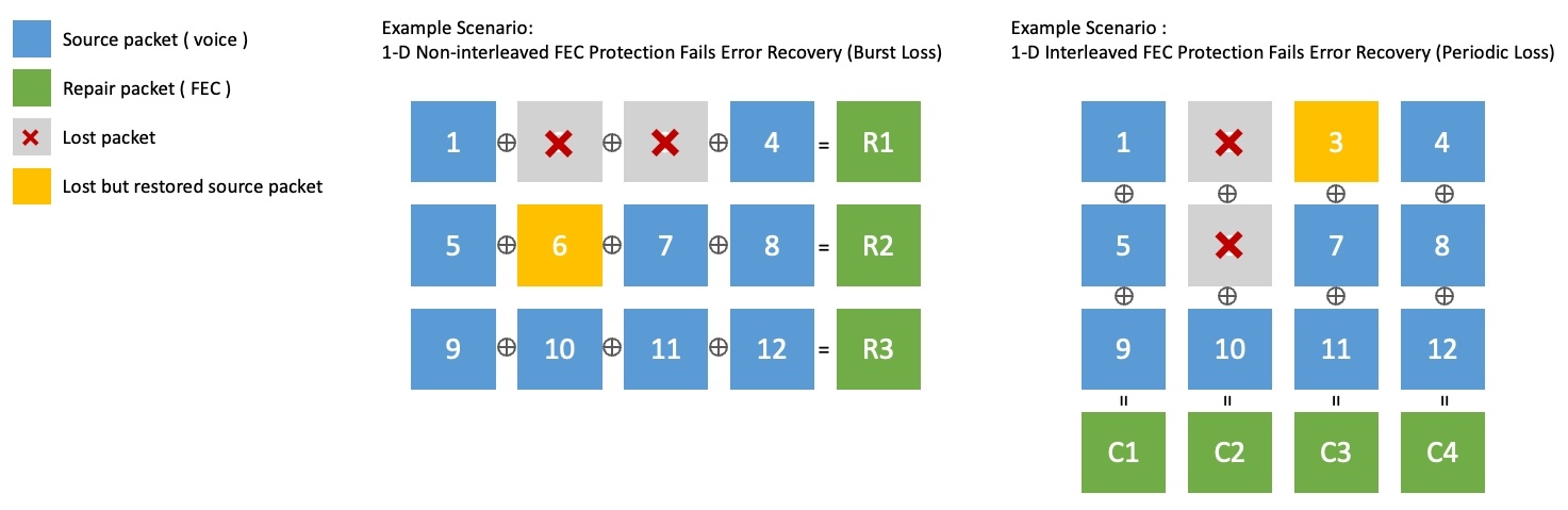
Single-dimensional FEC generates recovery packets by XOR operation of a group of source packets in row units (1-D non-interleaved) or column units (1-D interleaved). However, it has a limitation that it can't recover more than two consecutive packet losses. The following figure shows an example of this limitation.

• In 1-D Non-interleaved on the left in the figure below, packet 6 is recovered, but consecutive packet losses 2 and 3 can't be recovered.
• In 1-D Interleaved on the right in the figure below, packet 3 is recovered, but consecutive packet losses 2 and 6 can't be recovered.

2-D FEC Protection is a technology that combines single-dimensional Interleaved FEC and non-interleaved FEC. It can respond to various loss patterns, and with the iterative decoding algorithm, it can recover losses more effectively than general FEC. The figure below shows an example of using 2-D FEC Protection to recover all packets in two repetitions in the same situation as above.

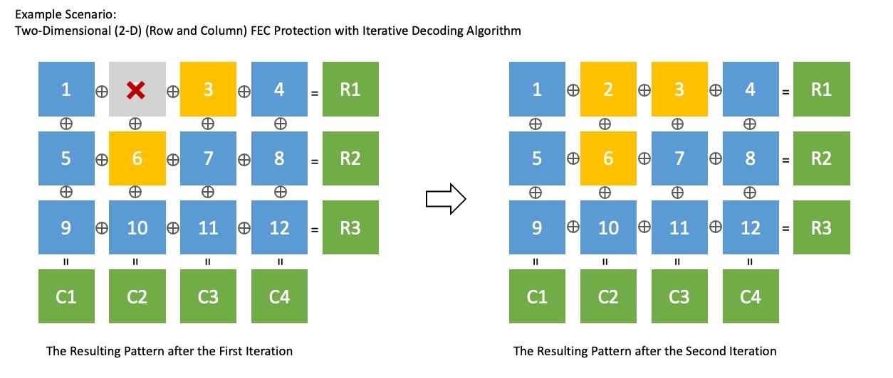
However, if the packet loss rate becomes very high, 2-D FEC Protection may not be enough. In such situations, we use a technique that periodically resends the same original packet two or more times. The sender side decides whether to use 2-D FEC Protection or periodic retransmission by monitoring the packet loss rate in real time.

Receiver side

On the receiver side, the lost packets are recovered using the recovery information transmitted by the sender. If there are still losses, a request is made for the lost packets to be resent. Retransmission causes delay, so it's limited not to operate in environments with high network latency. Finally, for voice sections where real-time packet loss recovery hasn't occurred, the degradation in sound quality is mitigated through PLC.

How to objectively evaluate voice quality

First, let's look at how to evaluate whether we are appropriately responding to packet loss and ensuring good voice quality. For this, we first need to be able to evaluate voice quality quantitatively and objectively, we need to measure one-way delay, and we need to check if the data usage is appropriate. Let's take a look at each one. 

Voice quality evaluation

MOS and subjective voice quality evaluation

Mean opinion score (MOS) is the most common measure used to evaluate the voice quality of voice calls or voice-based services. It's expressed on a scale from 1 to 5, with higher numbers indicating better voice quality. This method originated from the subjective quality measurement method, where people listen to the actual voice signal and subjectively evaluate the perceived sound quality.

The subjective evaluation of voice quality mainly uses the ITU-T P.800 recommendation. This recommendation also strictly regulates the environment for subjective evaluation. For example, the environment for recording and listening to evaluation sentences should have a space of 30-120 m³, a reverberation time of less than 500 ms (optimally 200-300 ms), and indoor noise of less than 30 dBA without peaks in the spectrum. In addition, evaluators shouldn't have participated in any subjective evaluations in the past six months, and in particular, they shouldn't have participated in listening subjective evaluations in the past year. There are also various conditions presented to remove deviations that may arise from evaluation conditions or environments. Therefore, subjective voice quality evaluation has the problem of inevitably requiring a lot of cost and time.

Objective voice quality evaluation and POLQA

To solve the problem of subjective voice quality evaluation, a method was needed to objectively evaluate voice quality. For this, various voice quality evaluation algorithms have been developed that provide evaluations similar to subjective quality measurement results by comparing with the original voice signal.

Among various algorithms, the widely used global standard algorithm is perceptual objective listening quality analysis (POLQA). This algorithm, standardized by the International Telecommunication Union - Telecommunication Standardization Sector (ITU-T), is widely used to evaluate the quality of voice services and codecs. POLQA evaluates sound quality by imitating the human auditory system when performing voice quality evaluation, and provide evaluations sound quality loss due to network environment changes such as network transmission, voice codec compression, packet loss, and delay.

Like subjective evaluation, POLQA also uses MOS as a measure of voice quality evaluation. This allows for the objective measurement and comparison of the quality of voice calls and voice services. Below is a sample MOS score evaluated by POLQA for actual sound sources. You can perceive the actual voice quality for each POLQA MOS score.

POLQA MOS	Sample audio
Original
4.5
3.5
2.5
1.5

Evaluating one-way delay

Even if the quality of the voice is good, if the one-way delay for the voice to be delivered is large, two-way communication can only be inconvenient. One-way delay is one of the important parameters in communication services such as VoIP or telephone calls, and it refers to the time it takes for the voice to depart from one point and arrive at its destination.

The standard recommendation for one-way transmission time, ITU-T G.114 (05/2003) One-way transmission time, recommends that one-way delay shouldn't exceed 400 ms in general networks. However, in some exceptions, this limit can be exceeded. For example, in a network environment with a high packet loss rate, it would be better for user experience to have some waiting time for packet loss recovery, even if the one-way delay is slightly longer, so that the loss can be somewhat recovered. Therefore, you need to measure the one-way delay to see if such loss recovery mechanisms are being properly controlled.

Evaluating data usage

Recently, with the advancement of mobile networks, voice data usage is often not a big issue. However, since the LINE app is used worldwide, it's necessary to consider cases where network performance is poor.

To recover packet loss, you need to use additional data. This can increase the bitrate, potentially causing network congestion. Especially for high bitrate media like video, you need to be more careful. Therefore, you need to measure data usage to check whether the data usage for loss recovery is appropriate.

How to measure voice quality in a packet loss environment

Now that we have a way to objectively evaluate voice quality, let's look at how to measure voice quality in an environment where packets are lost.

Voice quality and delay analysis

We use a professional voice quality analysis device (voice quality analyzer) for reliable and objective voice quality measurement. The digital speech level analyzer (DSLA) is a device that can measure call quality in communication equipment and networks. The DSLA injects the original voice signal as input to the sender's terminal and captures the voice signal played at the receiver's terminal to compare and analyze it with the original voice signal. After the analysis is completed, it provides various analysis results. As mentioned earlier, you can get objective results using the POLQA algorithm. In other words, you can measure POLQA MOS and voice one-way delay.

Packet loss model and emulation

In networks, packet loss occurs in various patterns due to reasons such as network congestion, router buffer overflow, signal interference. Among them, random packet loss is the most common packet loss pattern, where packets are randomly lost in the network. Also, burst packet loss refers to cases where multiple packets are lost consecutively. In this case, burst packet loss has various modeling methods, and various variables such as state and probability according to that state exist, so there are differences in the degree of loss occurrence depending on the model and variable. Therefore, when we test performance, we use a random packet loss pattern.

Also, we use a professional network emulator called PacketStorm for reliable and precise network emulation. Using this equipment, you can test performance not only for packet loss but also for various network transmission impairments such as delay, jitter, reordering, and throttling. If you only emulate a random packet loss pattern, you can also use other tools like Network Link Conditioner provided by macOS.

Measurement scenario

Let's look at the scenario of measuring the voice quality of two terminals in a packet loss environment.

Setting up the measurement environment

First, connect terminals A and B to the ports of the voice quality analysis device (DSLA), and then set up the network. Network transmission impairments can be applied to the uplink of the sender or the downlink of the receiver.

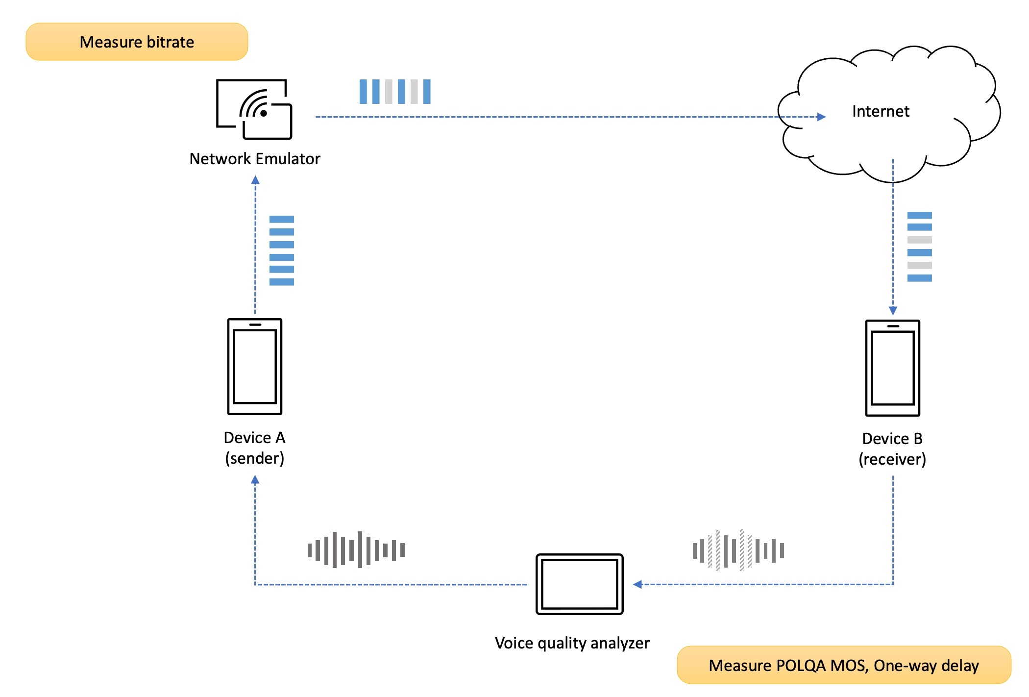
We measure both scenarios, and the figure above shows an example of applying the transmission impairment of packet loss to the uplink of the sender.

Connecting calls

Next, you need to connect the call. In the case of a LINE one-on-one call, the two terminals connect the call with each other, and in the case of a LINE group call, the two participants join the same group.

Measurement and analysis

Now start measuring voice quality and voice delay using the voice quality analysis device. Since random packet loss isn't always the same pattern, the measurement results of voice quality and voice delay can vary each time. Even in the same situation, the difference in MOS values can vary greatly depending on which section of the voice packet was lost. There may also be a difference in voice delay due to the delay that occurs while recovering lost packets. Therefore, it's good to repeat the DSLA test to increase the reliability of the evaluation data. We measure and analyze at least 50 times in one direction.

Analyzing measurement results

When the test is over, collect the results of voice quality (POLQA MOS), one-way delay of voice, and data usage. The collected results can be analyzed in various forms. For example, you can compare the distribution of MOS or delay measurement results depending on the loss rate, as shown below.

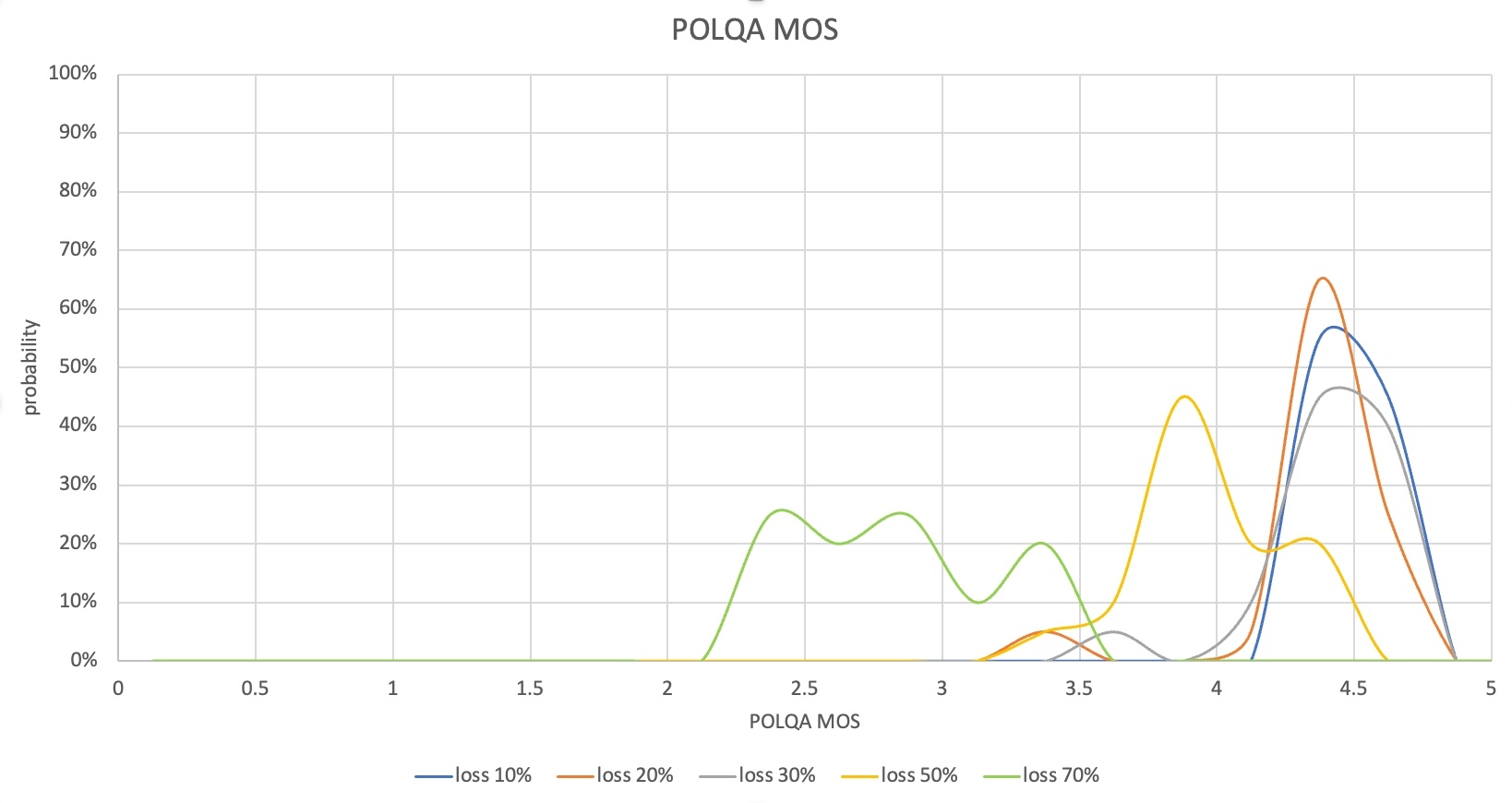
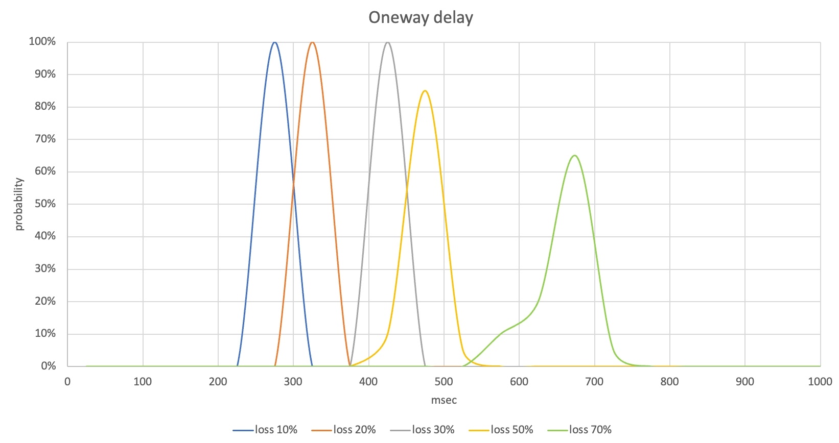
In this case, up to a 30% loss rate, the POLQA MOS distribution is 4-4.6, which indicates that most packet loss has been recovered. Since the one-way delay of the voice is also controlled to the early 400 ms, it's at a level that doesn't inconvenience the service. However, from a 50% loss rate, some voice sections were lost and the POLQA MOS was low, and at a 70% loss rate, there were many cases where the MOS was in the 2-point range, so you would feel uncomfortable in actual communication.

From the measurement results of this scenario, it can be confirmed that there is a need to improve loss recovery performance and reduce one-way voice delay from a loss rate of 50% or more. At this time, since data usage can increase for loss recovery, you need to analyze the data usage measurement results together.

Conclusion

In this article, we looked at what aspects we measure the call quality of the LINE app, and explained in detail how to measure AEC, frequency response, and loss robustness among various quality measurement methods. If we have the opportunity, we also plan to share other technologies and measurement methods that we couldn't introduce this time, including noise suppression.

We are committed to measuring and improving voice and video quality in various aspects using global standard evaluation algorithms, professional equipment, and our own technology so that LINE app users can enjoy excellent voice and video call experiences in any situation. We will continue to strive and improve so that users can experience the best call quality anytime, anywhere. Thank you for reading the long article.